MAGEMin_C iterative phase equilibrium calculations

Table of Contents

• Batch melting

  • 1. Create a new script

  • 2. Load and initialize

  • 3. Define pressure-temperature conditions

  • 4. Pre-allocate a vector of output structures

  • 5. Perform the calculations

  • 6. Accessing the results

  • 7. Plot the evolution of melt fraction

  • 8. Add other phase fractions

• Exercises

  • E.1. Add other mineral fraction evolution

  • E.2. Create plot for the evolution of heat capacity

  • E.3. Taking into account latent heat of reaction

  • E.4. Double y-axis plot

In the introduction, we have seen how to perform a single point calculation, how to access the results, and briefly how to visualize them. In this second part, we will focus on performing several calculations at fixed pressure and increasing temperature.

Batch melting

1. Create a new script

code MAGEMin_C_iterative_calculations.jl

2. Load and initialize

Like previously, let's load the necessary packages and initialize MAGEMin using the metapelite "mp" database:

using MAGEMin_C, Plots

data        =   Initialize_MAGEMin("mp", verbose=false);

X           = [0.5922, 0.1813, 0.006, 0.0223, 0.0633, 0.0365, 0.0127, 0.0084, 0.0016, 0.0007, 0.075]
Xoxides     = ["SiO2", "Al2O3", "CaO", "MgO", "FeO", "K2O", "Na2O", "TiO2", "O", "MnO", "H2O"]
sys_unit    = "wt"

3. Define pressure-temperature conditions

Let's first define a fixed pressure:

P = 5.0

Now let's define the temperature range over which we want to model batch partial melting:

T_step = 10.0
T = [600:T_step:1000;]

Here, the ";" at the end of the range directly converts the range into a vector!

4. Pre-allocate a vector of output structures

In order to improve efficiency and collect all the outputs from the temperature steps, we can pre-allocate the memory space.

First let's find the number of points we plan to calculate:

n_calc = length(T)

...and subsequently declare the vector of output structures:

Out_XY      = Vector{out_struct}(undef,n_calc)

5. Perform the calculations

Let's now create a loop of single point minimization to iterate over the defined temperature range:

for i in 1:n_calc
    Out_XY[i] = single_point_minimization(P, T[i], data, X=X, Xoxides=Xoxides, sys_in=sys_unit, name_solvus = true)
end

6. Accessing the results

Once the calculations have been performed, you can access the output of each individual calculation as

Out_XY[i]

where "i" is the index of the calculation.

Because the results of each calculation are stored in a vector of structures, we need a way to extract the needed information and create vectors/matrices out of them.

Let's first extract the evolution of the melt fraction across the temperature range:

melt_wt = [Out_XY[i].frac_M_wt for i=1:n_calc]

The previous command simply creates a vector by accessing "frac_M_wt" for every index of the output vector. Other possible and perhaps more explicit ways to achieve the same goal could be:

melt_wt = []
for i=1:n_calc
    push!(melt_wt,Out_XY[i].frac_M_wt)
end

or

melt_wt = zeros(Float64,n_calc)
for i=1:n_calc
    melt_wt[i] = Out_XY[i].frac_M_wt
end

7. Plot the evolution of melt fraction

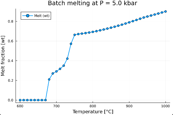
We can now visualize how the melt weight fraction evolves with temperature:

plot(T, melt_wt,
    xlabel      = "Temperature [°C]",
    ylabel      = "Fraction [wt]",
    title       = "Batch melting at P = $(P) kbar",
    label       = "Melt",
    markershape = :circle,
    markersize  = 4,
    linewidth   = 2,
    legend      = :topleft)

which gives:

8. Add other phase fractions

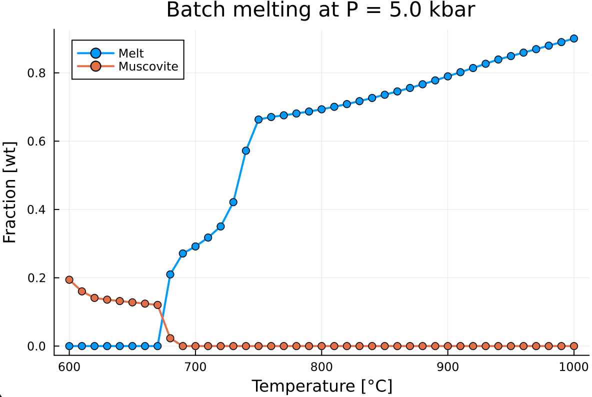
For instance, let's retrieve the evolution of the muscovite wt fraction:

mu_wt = zeros(Float64, n_calc)
for i=1:n_calc
    id_mu = findfirst(Out_XY[i].ph .== "mu")
    if !isnothing(id_mu)
        mu_wt[i] = Out_XY[i].ph_frac_wt[id_mu]
    else
        continue
    end
end

Here, we pre-allocate the mu_wt vector with zeros and loop through all points to check if mu is stable. If mu is stable (id_mu is not nothing), we then fill the array with ph_frac_wt[id_mu].

Now we add mu_wt to the previous plot:

plot!(T, mu_wt,
    label       = "Muscovite",
    markershape = :circle,
    markersize  = 4,
    linewidth   = 2,
    legend      = :topleft)

which gives:

Exercises

E.1. Add other mineral fraction evolution

• Similarly to muscovite, add plagioclase pl and biotite bi wt fraction evolution to the previous diagram.

E.2. Create plot for the evolution of heat capacity

• Create a new plot where you display the evolution of heat capacity Out_XY[i].s_cp. Note that s_cp is stored as a vector of size one, and to access the value you need to use Out_XY[i].s_cp[1].

• What do you notice?

E.3. Taking into account latent heat of reaction

• In the previous exercise, we have seen that the specific heat capacity did not account for latent heat of reaction. Heat capacity is computed as a second-order derivative of the Gibbs energy with respect to temperature using numerical differentiation:   There are, however, two ways to retrieve the second-order derivative:

  1. Default option scp = 0 — no latent heat of reaction: fixing the phase assemblage (phase proportions and compositions) and computing the Gibbs energy of the assemblage at T, T+eps and T-eps.

  2. Full differentiation option scp = 1 — latent heat of reaction: computing three stable phase equilibria at T, T+eps and T-eps.

In order to account for latent heat of reaction, you simply need to rerun the calculation while modifying the `single_point_minimization()` call to:

for i in 1:n_calc
    Out_XY[i] = single_point_minimization(P, T[i], data, X=X, Xoxides=Xoxides, sys_in=sys_unit, name_solvus = true, scp=1)
end

which will give you something like:

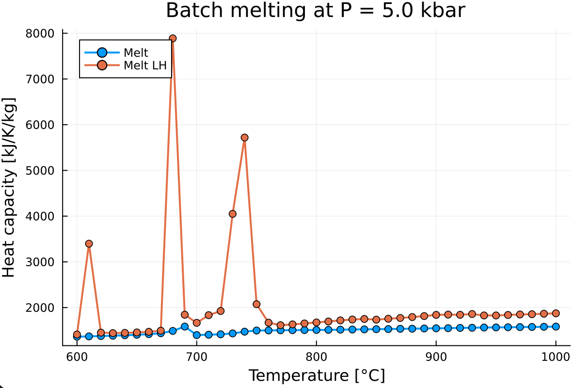
• As you can notice, the evolution of the specific heat capacity with latent heat of reaction is rather spiky. To fix this, increase the resolution of the calculation by decreasing T_step from 10.0 to 1.0.

• This will largely increase the calculation time. In order to track the progress of the calculation, add a new package to your local environment:

] add ProgressMeter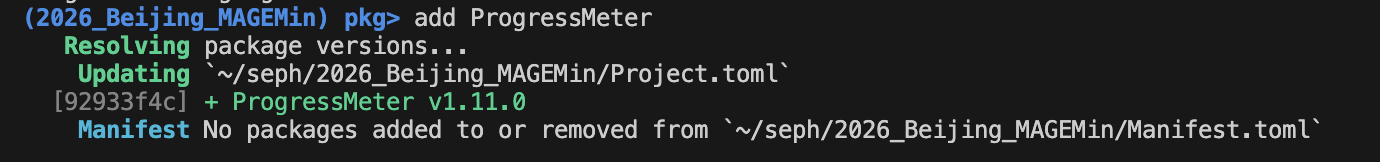

• Add ProgressMeter to the list of packages at the beginning of your script

using MAGEMin_C, Plots, ProgressMeter

• Add @showprogress at the beginning of your calculation loop to activate the progress bar:

@showprogress for i in 1:n_calc
    Out_XY[i] = single_point_minimization(P, T[i], data, X=X, Xoxides=Xoxides, sys_in=sys_unit, name_solvus = true, scp=1)
end
s_cp = [Out_XY[i].s_cp[1] for i=1:n_calc]

• Re-running the calculation should now display the progress bar:

E.4. Double y-axis plot

• To better visualize the relationship between the evolution of melt fraction and the specific heat capacity (with latent heat) create a twin plot from your previous high resolution calculation. This can be done using the following plot script:

p = plot(T, s_cp,
    xlabel      = "Temperature [°C]",
    ylabel      = "Heat capacity [J/K/kg]",
    label       = "Cp",
    linewidth   = 2,
    legend      = :topleft,
    color       = :blue,
    dpi         = 300)

# Right y-axis: melt fraction
plot!(twinx(p), T, melt_wt,
    ylabel      = "Melt fraction [wt]",
    label       = "Melt",
    linewidth   = 2,
    legend      = :topright,
    color       = :red)

• Notice that here we add the plot in "p" variable. This allow to save the plot using:

savefig(p, "scp_vs_melt.png")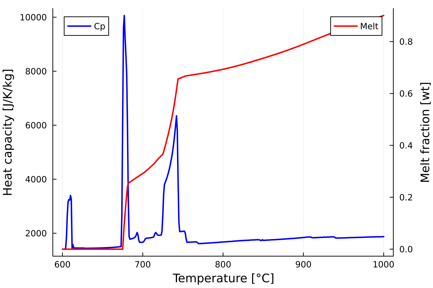

• What is the relationship between melt fraction evolution and latent heat of reaction?

• What is happening at sub-solidus? (~610 °C)