MAGEMin_C Li partitioning

Table of contents

• Batch melting equations

  • 1. Create a new script

  • 2. Initialize

  • 3. Define partition coefficients

  • 4. Define starting mass fraction and partition coefficient database

  • 5. Perform stable phase equilibrium calculation

  • 6. Perform trace-element prediction modelling

  • 7. Access result of trace-element partitioning

  • 8. Visualize Li enrichment

• Exercises

  • E.1. Batch melting

  • E.2. Extract mineral Li enrichment

  • E.3. Different set of partition coefficients

• The objective of this tutorial is to demonstrate how to add trace-element partitioning to stable phase equilibrium predictions. As an example, we will model Li partitioning during partial melting of a metapelite using the metapelite mp database (White et al., 2014).

• The partition coefficients used to predict partitioning between minerals and melt are taken from two studies: Ballouard et al. (2023) and Koopmans et al. (2024).

Mineral	Acronym	K_D BA	K_D KO
Alkali-feldspar	afs	1e-4	0.01
Amphibole	amp	1e-4	1e-4
Biotite	bi	0.55	1.67
Clinopyroxene	cpx	1e-4	1e-4
Cordierite	cd	1.10	0.44
Garnet	g	0.09	1e-4
Hematite	hem	1e-4	1e-4
Ilmenite	ilm	1e-4	1e-4
Kyanite	ky	1e-4	1e-4
Magnetite	mt	1e-4	1e-4
Muscovite	mu	0.11	0.82
Orthopyroxene	opx	1e-4	1e-4
Plagioclase	pl	1e-4	0.02
Quartz	q	1e-4	1e-4
Rutile	ru	1e-4	1e-4
Sillimanite	sill	1e-4	1e-4

BA = Ballouard et al., 2023; KO = Koopmans et al., 2024

Batch melting equations

To predict the mass content of Li in both the solid and liquid phases, MAGEMin uses trace-element batch melting equations (Shaw, 1970; Hertogen & Gijbels, 1976; Zou, 2001):

and

where and are the mass contents of trace element in the melt and solid in μg/g, respectively, is the initial mass content of element in the bulk rock, is the melt weight fraction, and is the whole-rock bulk partition coefficient defined as:

where is the weight fraction of mineral m/melt, and is the mineral/melt partition coefficient for element in mineral m/melt. The mass content for element in mineral m () is retrieved as:

1. Create a new script

code MAGEMin_C_Li_partitioning.jl

2. Initialize

Let's first initialize MAGEMin using the world median pelite composition:

using MAGEMin_C, Plots, ProgressMeter
dtb         = "mp"
data        =  Initialize_MAGEMin(dtb, verbose=false);

X           = [0.5922, 0.1813, 0.006, 0.0223, 0.0633, 0.0365, 0.0127, 0.0084, 0.0016, 0.0007, 0.075]
Xoxides     = ["SiO2", "Al2O3", "CaO", "MgO", "FeO", "K2O", "Na2O", "TiO2", "O", "MnO", "H2O"]
sys_unit    = "wt"

P           = 5.0
T           = 700.0

3. Define partition coefficients

Let's now define the lithium partition coefficients between minerals and melt using Koopmans et al. (2024) values:

el          = ["Li"]
ph          = ["afs", "amp", "bi", "cpx", "cd", "g", "hem", "ilm", "ky", "mt", "mu", "opx", "pl", "q", "ru", "sill"]
KDs         = ["0.01";  "1e-4";  "1.67"; "1e-4";  "0.44"; "1e-4"; "1e-4"; "1e-4";  "1e-4"; "1e-4"; "0.82"; "1e-4";  "0.02"; "1e-4"; "1e-4"; "1e-4"]

• Here, KDs is a Matrix of String of size (n_ph, n_el):

KDs	el_1	el_2	...	el_m
ph_1	KD_1,1	KD_1,2	...	KD_1,m
ph_2	KD_2,1	KD_2,2	...	KD_2,m
...	...	...	...	...
ph_n	KD_n,1	KD_n,2	...	KD_n,m

where n is the total number of phases and m is the total number of trace elements.

4. Define starting mass fraction and partition coefficient database

Then, we need to define the starting mass fraction and create the custom partition coefficients database:

C_te        = [400.0]       #starting mass fraction of elements in ppm (ug/g)
KDs_dtb     = create_custom_KDs_database(el, ph, KDs)

5. Perform stable phase equilibrium calculation

Let's now compute the stable equilibrium (without trace-element prediction):

out  = single_point_minimization(P, T, data, X=X, Xoxides=Xoxides, sys_in=sys_unit, name_solvus = true)

6. Perform trace-element prediction modelling

We can now compute trace-element partitioning by calling the TE_prediction() function, while passing the result of the minimization out, the starting mass fraction C_te, the partition coefficient database KDs_dtb, and the database name dtb as arguments:

out_TE = TE_prediction(out, C_te, KDs_dtb, dtb)

7. Access result of trace-element partitioning

Results of trace-element prediction are stored in the out_TE structure:

out_TE.
C0            Cliq          Cmin          Csol
Sat_P2O5_liq  Sat_S_liq     Sat_Zr_liq    bulk_D
bulk_cor_mol  bulk_cor_wt   elements      fapt_wt
liq_wt_norm   ph_TE         ph_wt_norm    sulf_wt
zrc_wt

The melt lithium mass fraction is stored in:

out_TE.Cliq
1-element Vector{Float64}:
 714.3816978649379

The mineral phases hosting Li are listed in:

out_TE.ph_TE
5-element Vector{String}:
 "pl"
 "hem"
 "bi"
 "q"
 "sill"

and the lithium mass fraction of these phases is stored in:

out_TE.Cmin
5×1 Matrix{Float64}:
  14.287633957298759
   0.0714381697864938
1193.0174354344463
   0.0714381697864938
   0.0714381697864938

8. Visualize Li enrichment

The variations in lithium mass fractions are best visualized by normalizing to the starting mass out_TE.C0. To achieve this, let's create a bar graph:

First, combine phase names and melt:

labels = [out_TE.ph_TE; "melt"]

Then, combine mineral and melt Li concentrations:

Li_norm = [out_TE.Cmin[:, 1]; out_TE.Cliq[1]] ./ out_TE.C0

• Note that out_TE.Cmin is a matrix, while out_TE.Cliq is a vector of length 1.

bar(labels, Li_norm,
    ylabel    = "Li norm [Li/Li₀]",
    title     = "Li partitioning at P = $(P) kbar, T = $(T) °C",
    legend    = false,
    xrotation = 45,
    color     = reshape(1:length(labels), 1, :))

hline!( [1.0],
        linestyle   = :dot,
        linecolor   = :black,
        label       = "C0")

This gives:

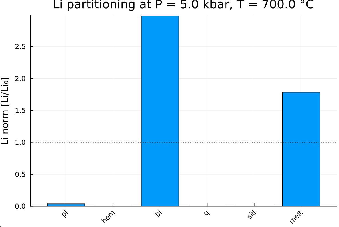
• The horizontal dashed line at 1.0 represents the starting mass fraction.

Exercises

E.1. Batch melting

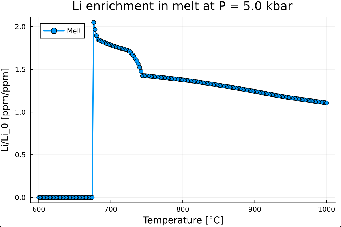
• Using the previous tutorials on batch melting, duplicate this script and modify it to perform Li partitioning prediction between 600 and 1000.0 °C with a step of 2 °C.

  • Remember to pre-allocate the out and out_TE structures as: julia Out_XY = Vector{out_struct}(undef,n_calc) Out_TE_XY = Vector{out_TE_struct}(undef,n_calc)

• Extract the Li mass fraction in the liquid, normalize it using the initial mass fraction, and visualize the result. This gives:

• Perform the same calculation at various pressures (2.0, 4.0, 8.0, and 12.0 kbar). How does pressure control the maximum lithium enrichment of the melt?

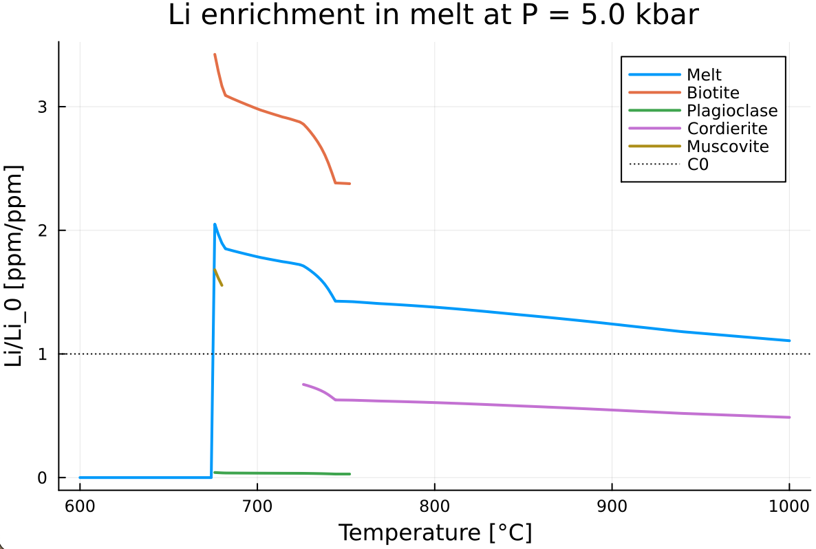
E.2. Extract mineral Li enrichment

• Create a function that reads the trace-element output structure Out_TE_XY, the starting Li mass fraction, a Li-bearing mineral name, and returns a vector of Li enrichment:

function get_Li_enrichment(Out_TE_XY, C0, phase)
#... make the function yourself ...
return Li_ratio_phase
end

• Plot the evolution of the lithium enrichment of melt, biotite, plagioclase, cordierite, and muscovite. This should give something similar to:

• Now add as a twinx(), the evolution of the melt fraction in wt

• What is the relationship between Li enrichment in the melt, biotite and melt fraction?

E.3. Different set of partition coefficients

• Let's now use a different set of partition coefficients. Modify your script to add an option for choosing between KO (Koopmans et al., 2024) and BA (Ballouard et al., 2023)

• Perform the calculation using BA set of partition coefficients

• How does this change the maximum Li enrichment in the melt? How do you explain it?

• Compare Li enrichment prediction between BA and KO sets at various pressures. How important is the choice of partition coefficients?