P-T-X paths tutorials (MAGEMinApp v1.2.1)

Here we provide a set of tutorials to generate various kind of pressure-temperature-composition paths: including batch melting, fractional melting and fractional crystallization.

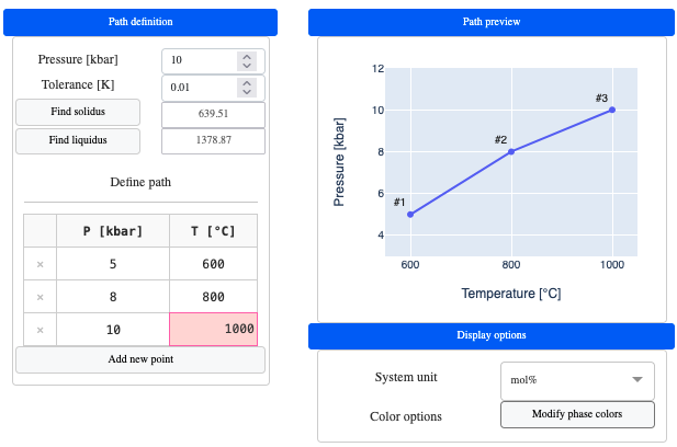
E.1. Quick start - first P-T-X path

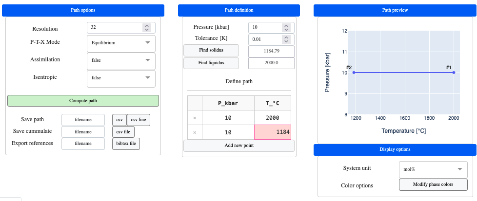
For the first P-T-X path, simply launch MAGEMinApp and navigate to the PTX path tab. Change default setting for the thermodynamic database (Igneous)(Green et al., 2025 after Holland et al., 2018) and default bulk-rock composition (KLB1 Peridotite anhydrous). In the Path definition panel click on Find solidus and Find liquidus and define the P-T points accordingly:

Note

• New points for the P-T-X path can be added by clicking on Add new point.

• To delete a point simply click on the cross icon on the left of point.

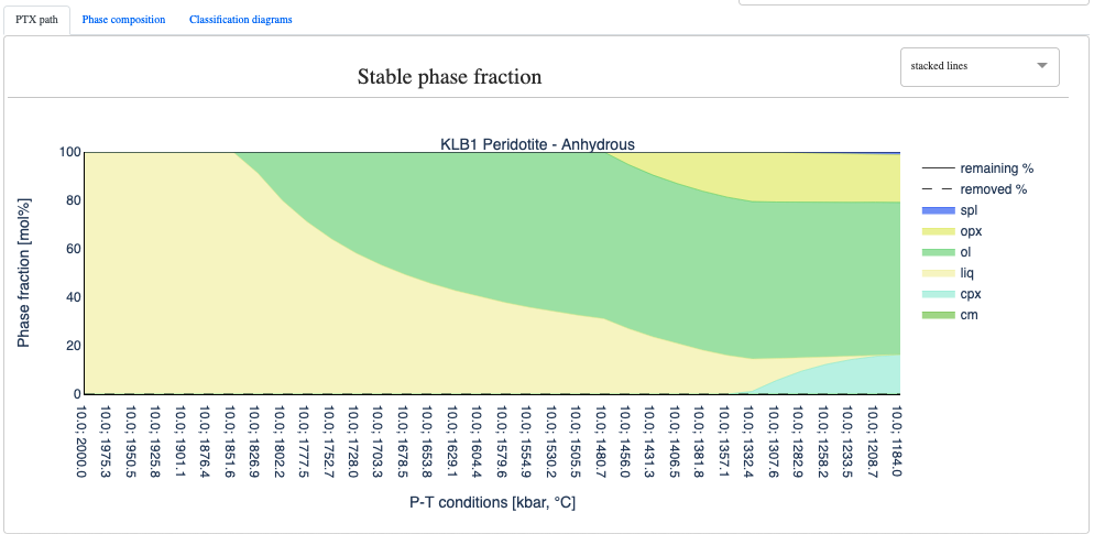
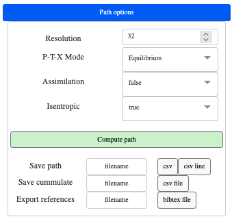
In the Path options panel, change the resolution to 32. This option defines the number of point-wise calculation between two defined points. Hit Compute path and after a few seconds you should get the following result:

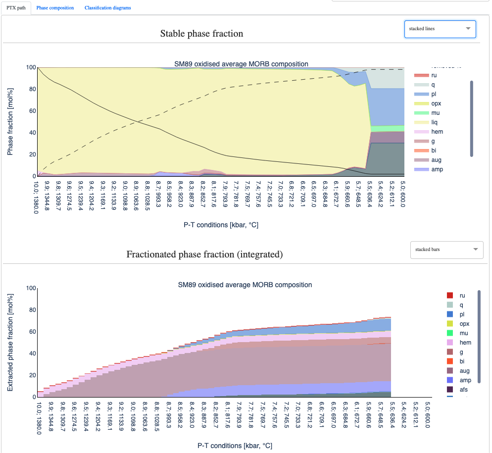
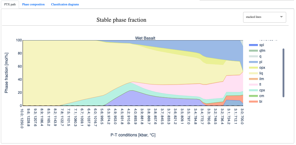
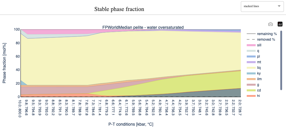
Stable phase fraction

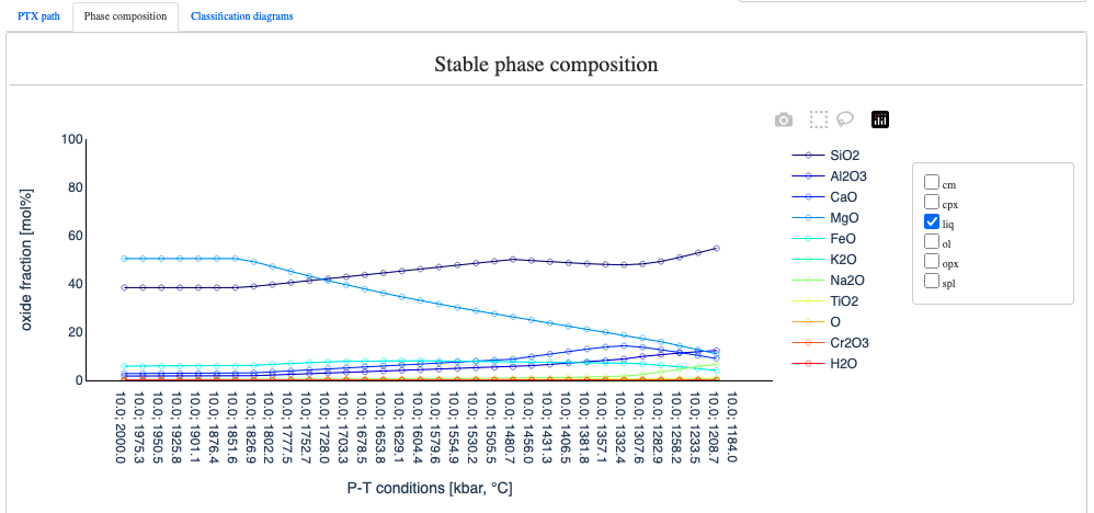
Stable phase composition

Then in the Phase composition tab, click liq which will display the evolution of the melt composition along the path:

Note

• Double-clicking on one ooxide will isolate it.

• Double-clicking again on the same oxide, will bring back all the oxides.

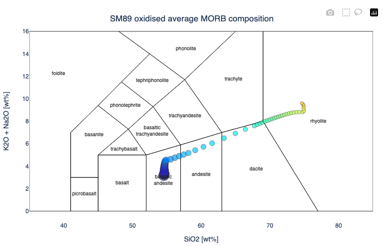
TAS diagram

When liq is selected you can access the TAS diagram which displays the evolution of the melt composition (Total Alkali Silica):

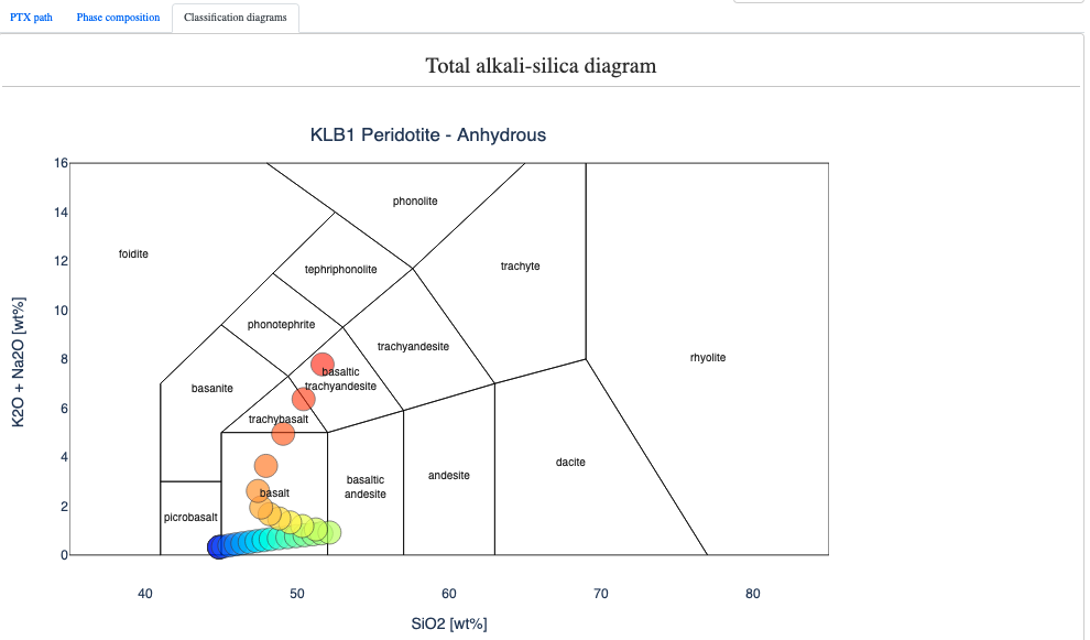
Warning

• When computing a new PTX diagram, to refresh the TAS diagram, you need to unselect and reselect liq in the Composition panel.

E.2. Fractional melting

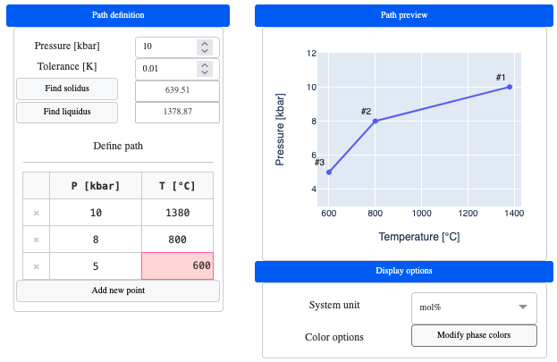
In this example, we are going to perform fractional melting using SM89 oxidized average MORB composition using the Metabasite thermodynamic database (Green et al., 2016). First make sure you select Aug in the clinopyroxene selection, then define the P-T points of the path as follow:

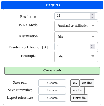
In the Path options panel, choose a resolution of 32, and select P-T-X mode = fractional melting, keep Assimiliation = false and Connectivity threshold [%] = 7:

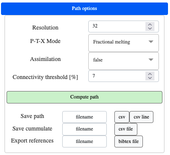
Note

• The connectivity threshold is the value above which melt is extracted

• Presently, only the melt above this value is extracted to keep the melt fraction at the connectivity threshold.

• When computing a fractional melting path using a connectivity threshold, the displayed fraction of melt can be slightly above the threshold as the removed fraction of melt is only applied to the subsequent calculation step. This effect can however be minimized by increasing the resolution.

Process with the P-T-X path calculation, which should yield:

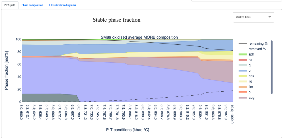
Note

• The black continuous line remaining % represents the remaining % with respect to the starting material.

• The black dashed line removed % is the mass % of material removed with respect to the starting material.

• remaining % + removed % = 100.0

E.3. Fractional crystallization

Let us the same database and bulk rock composition as for the fractional melting example. Simply change the path definition as follow:

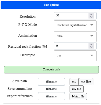
In the Path options panel, choose a resolution of 32, and select P-T-X mode = fractional crystallization, keep Assimiliation = false and Remaining fraction [%] = 1:

Note

• Remaining fraction [%] can be thought as a small fraction of the solid rock carried by the fractionating melt.

Process with the P-T-X path calculation, which should yield:

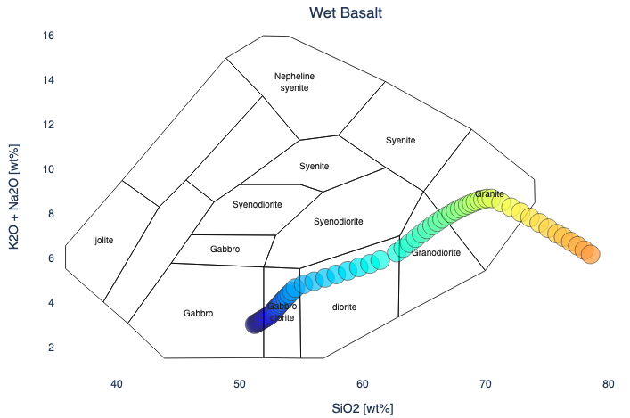
and TAS diagram (Total Alkali Silica):

Note

• The size of the circle symbol in the TAS diagram scales with the remaining %. This gives an idea of the volume of generated magma along the fractional crystallization path.

E.4. Assimilation

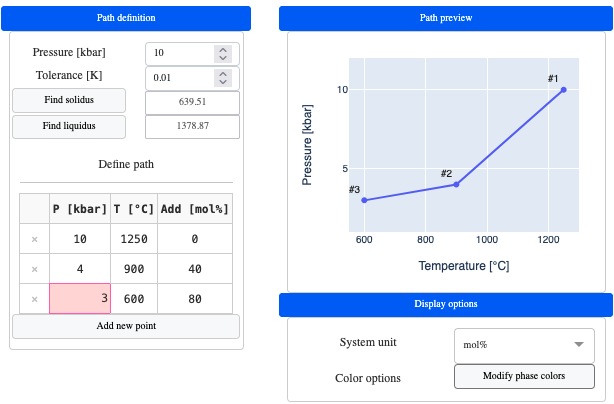
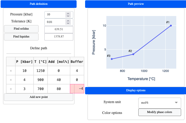
In this example we are going to compute an equilibrium batch crystallization path of a wet basalt, and, progressive assimilation of tonalitic composition. Let's first select the Igneous database (Green et al., 2025, after Holland et al., 2018) and define the P-T path as follow:

Note

• Notice the new column in the P-T path definition Add [mol%]. Here you can define how much of the assimilated composition will be added for each P-T step.

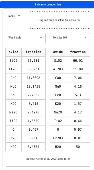
In Path options, set Resolution = 32, P-T-X mode = Equilibrium and Assimilatiom = true. When Assimilatiom = true a second bulk-rock composition is available for selection in the Bulk-rock compositionleft panel. Choose Wet basalt for the left (starting) composition and Tonalite 101 for the right (assimilated) composition:

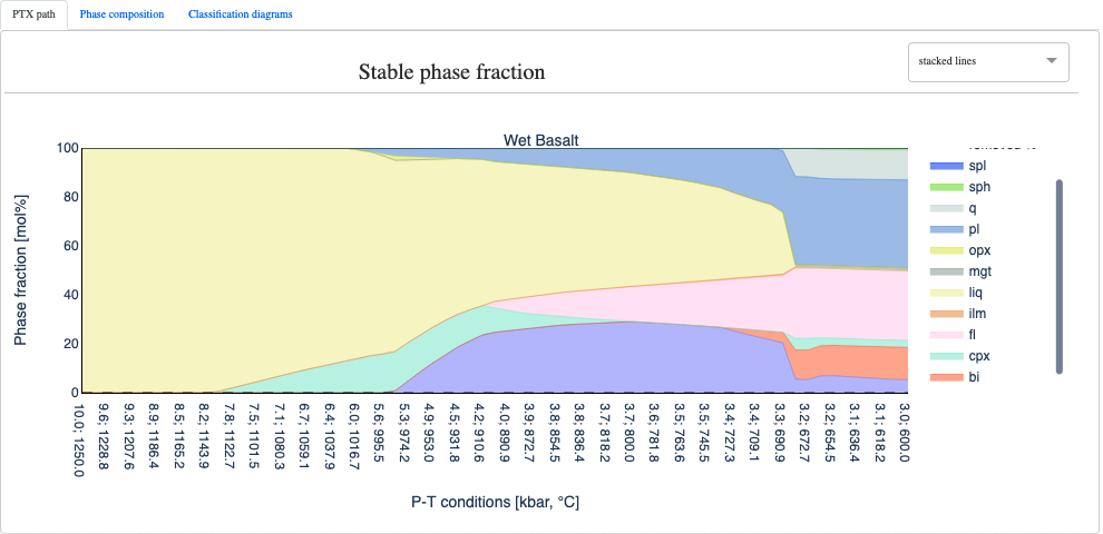
Performing the calculation of the P-T path gives:

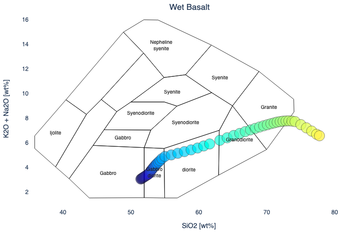
and the following TAS diagram:

E.5. Variable buffer

To simulate a change in oxydation/reduction state of the system you can also provide variable buffer offsets. Let's start from previous assimilation example 4, and select Buffer = QFM and Variable buffer = true in the Configuration panel.

A new column named Buffer is now available in the Path definition panel and you can modify the buffer offset to your liking. For instance:

Tip

Don't forget to oversaturate the O content of the bulk-rock compositions.

Performing the calculation of the P-T path gives:

and the following TAS diagram:

Isentropic path (MAGEMinApp v1.2.1)

Isentropic path typically represent a process where a rock or material undergoes changes in pressure and temperature without any exchange of heat with its surroundings (adiabatic process) and without any entropy production (reversible process). This type of path is often used to model processes like mantle convection or adiabatic decompression melting, where material moves through the Earth's interior under conditions that approximate constant entropy.

Note

The isentropic tab was removed in MAGEMinApp@1.2.1 and merged with PTX path tab. This allowed to use the PTX functionality such as fractional crystallization and assimilation

E.6. Isentropic path - constant bulk

Isentropic paths are easy to setup. Simply launch MAGEMinApp and navigate to the PTX path tab. Change to thermodynamic database (Metapelite)(White et al., 2014) and default bulk-rock composition. In the Path options panel, select Isentropic = true and keep all other parameters by default:

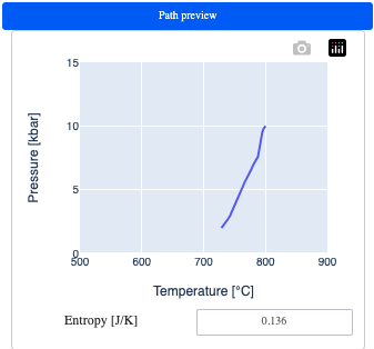
Notice here that for isentropic path only the starting temperature and pressure can be changed. Then simply click Compute path:

Note

• Here we use a bisection method to ensure constant entropy within a temperature tolerance

• In the top-right panel (Path preview ) you can retrieve information about the entropy value in J/K and the isentropic pressure-temperature path.

E.7. isentropic fractional crystallization

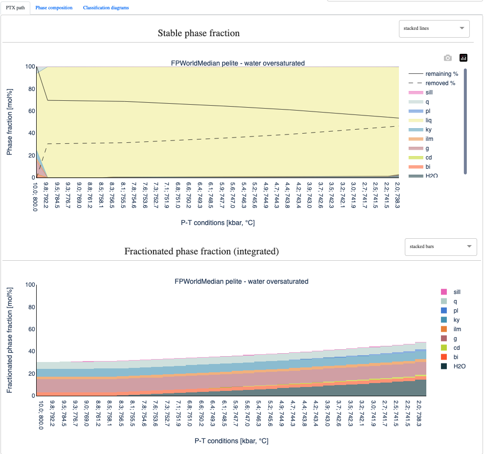
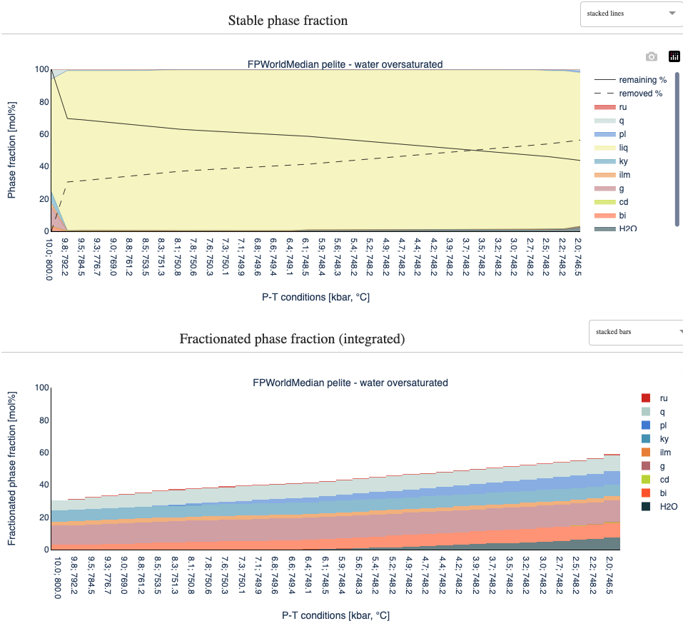
Building upon previous example, you can use the fractional crystallization mode along with the isentropic option:

Computing the path will generate two diagrams: the stable phase fractions and fractionated phases.

E.8. isentropic fractional crystallization with assimilation

One can also compute isentropic crystallization paths with assimilation of a secondary bulk-rock composition (host-rock, second magma etc.)

First activate the Assimilation option. Then, in the Path definition panel, you can see that next to pressure a new column appears which allows you to add fraction of the second bulk-rock composition in mol%. Modify the entry for the second point to 50%:

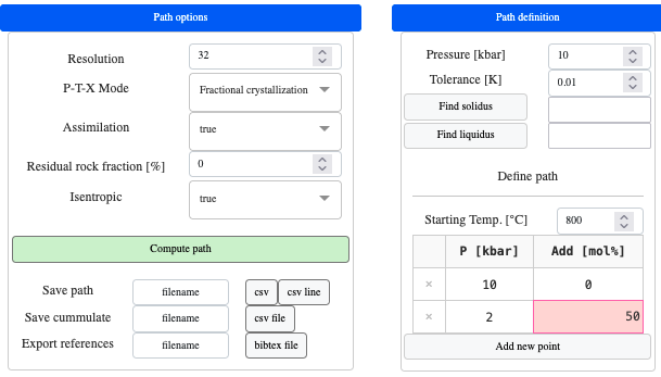
Note

• If you put a non zero value for the first row of the Add [mol%] column this will change the starting bulk-rock composition accordingly

• When changing any other rows, the Add [mol%] will be added progressively from the previous point

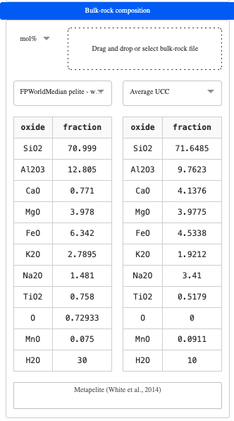
You can now change the second bulk-rock compositon available in the left Bulk-rock composition panel. For instance:

Compute the path:

Modify colormap (MAGEMinApp v1.2.1)

Since version 1.2.0 it is possible to adjust the colormap of the area plots. In the Display options panel on the right, click on Modify phase colors:

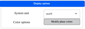
This unfold a window a the left of your screen where the colors of all stable phases are displayed:

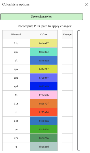
To modify a color, click the corresponding cell in the Change column, then change the thin colored bar on the right. This option the color picker:

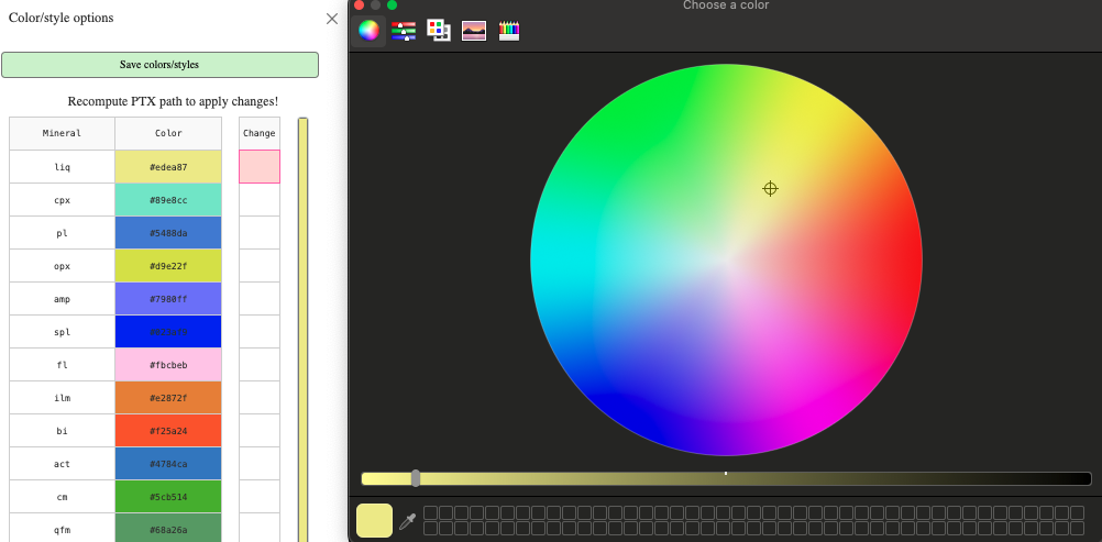
Note

• Only the phases stable in your calculation can be modified

• Once your happy with the updated colors, to apply the changes, you need to redo the PTX path calculation

• You can save your changes by clicking on the green button Save colors/styles. The changes are saved even when restarting the App.

Trace-element partitioning (MAGEMinApp v1.5.1)

Trace-element (TE) partitioning can be computed simultaneously with any P-T-X path (batch melting, fractional melting, fractional crystallization, isentropic). The module uses lattice-strain parameterized Kd databases and optionally applies mineral or volatile saturation models (Zr, S, P₂O₅, CO₂).

E.9. Trace-element partitioning setup

Step 1 — Activate the TE predictive model

In the Path options panel, set TE predictive model = true. This reveals the Trace Elements panel in the left sidebar.

Step 2 — Configure KD model and saturation options

In the Trace Elements panel, the following options are available:

Option	Description	Available values
KD model	Lattice-strain Kd database	OL — O. Laurent (2012) ; CO — J. Cornet (2019)
Zr saturation	Zircon saturation model	none ; Watson 1979 (WH) ; Blundy 2022 (CB)
S saturation	Sulfide saturation model	none ; Liu 2021 (Liu07)
P₂O₅ saturation	Fluorapatite saturation model	none ; Tollari 2006
CO₂ saturation	CO₂ fluid saturation model	none ; SY26 — Sun & Yao (2026)

Note

• Saturation models only activate when the corresponding element is present in the TE bulk composition.

• The CO₂ saturation model (SY26) requires dissolved H₂O in the melt: it inverts the H₂O solubility equation to derive P_H₂O, then evaluates CO₂ solubility at P_CO₂ = P − P_H₂O.

Step 3 — Load the trace-element bulk composition

Two options are available:

• Built-in database: use the dropdown below the saturation options to select a predefined TE composition; the Initial TE bulk composition [μg/g] table updates automatically.

• Custom file: drag and drop a CSV file onto the upload area. The file must contain element and μg/g columns.

Values in the table are editable directly in the interface.

When Assimilation = true, a second table (Assimilant TE bulk composition [μg/g]) is also displayed and follows the same loading logic.

Step 4 — Compute the path

Click Compute path. Thermodynamic minimization and TE partitioning are performed simultaneously at each step along the path.

E.10. Visualizing trace-element results

After computation, the Trace Elements tab becomes enabled. It contains:

• REE spectrum (top panel): rare-earth element pattern at the selected path point, normalized to bulk or chondrite. Use the Show dropdown to switch between ree (REE only) and all (extended trace-element set).

• Diagram (bottom panel): P-T diagram colored by a user-selected TE or saturation field.

In the Display options panel (right side) use the Field type dropdown to choose what to display:

Field type	Available fields
Zircon	Sat_Zr_liq [ug/g] — Zr saturation in melt ; zrc_wt — zircon weight fraction
Sulfide	Sat_S_liq [ug/g] — S saturation in melt ; sulf_wt — sulfide weight fraction
Fluorapatite	Sat_P2O5_liq [ug/g] — P₂O₅ saturation in melt ; fapt_wt — apatite weight fraction
CO2 saturation	Sat_CO2_liq [ug/g] — CO₂ saturation in melt ; fl_CO2_wt — CO₂ fluid weight fraction
Trace element	Any TE concentration or user-defined expression (see below)

For the Trace element field type, the Field builder allows you to enter arbitrary expressions, for example:

• [M_Dy] / [M_Yb] — Dy/Yb ratio in the melt

• [M_La] / [M_Sm] — La/Sm ratio

where [M_X] refers to element X in the melt. Set a normalization (none, bulk, chondrite) and click Compute and display.

Isopleths (contour lines) for any field can be added from the Isopleths tab: select the field type and field, set the range and step, and click Add.

E.11. Exporting trace-element results to CSV

When TE predictive model = true, additional export buttons appear in the Path options panel:

Button	Filename field	Content
Save path → csv	Save path input	Full PTX path: P, T, phase fractions and oxide compositions at each step (one row per step)
Save path → csv line	Save path input	Same content but all steps written on a single row (useful for batch processing)
Save cumulate → csv file	Save cumulate input	Cumulate (extracted solid) composition along the path
Save trace elements → csv file	Save trace elements input	TE concentrations in the melt, bulk solid and individual mineral phases at each step
Save cumulate TE → csv file	Save cumulate TE input	Integrated cumulate TE composition at each step

Note

• Save trace elements and Save cumulate TE are only active after trace elements have been computed. A warning badge is shown if you try to export beforehand.

• All CSV files are saved to the output/ subdirectory of the working directory displayed in the Julia terminal.

Tip

Use the Export references → bibtex file button to export a BibTeX file listing all references for the active KD model, saturation models and thermodynamic database.