MAGEMin_C.jl: Fractional crystallization

This tutorial demonstrates how to perform fractional crystallization using MAGEMin_C.jl, from a hydrous basalt starting composition along a cooling and decompression path, with visualization of melt composition and density evolution.

Info

• Fractional crystallization

Note

• This tutorial is not optimized for performance, but is provided in the hope it can be useful to present MAGEMin_C functionality.

Fractional crystallization

The following example shows how to perform fractional crystallization using a hydrous basalt magma as a starting composition. The results are displayed using PlotlyJS. This example is provided in the hope it may be useful for learning how to use MAGEMin_C for more advanced applications.

Note

Note that if we wanted to use a buffer, we would need to initialize MAGEMin as in example 4. Because during fractional crystallization the bulk-rock composition is updated at every step, we would need to increase the oxygen-content (O) of the new bulk-rock

using MAGEMin_C
using PlotlyJS

# number of computational steps
nsteps = 64

# Starting/ending Temperature [°C]
T = range(1200.0,600.0,nsteps)

# Starting/ending Pressure [kbar]
P = range(3.0,0.1,nsteps)

# Starting composition [mol fraction], here we used an hydrous basalt; composition taken from Blatter et al., 2013 (01SB-872, Table 1), with added O and water saturated
oxides  = ["SiO2"; "Al2O3"; "CaO"; "MgO"; "FeO"; "K2O"; "Na2O"; "TiO2"; "O"; "Cr2O3"; "H2O"]
bulk_0  = [38.448328757254195, 7.718376151972274, 8.254653357127351, 9.95911842561036, 5.97899305676308, 0.24079752710315697, 2.2556006776515964, 0.7244006013202644, 0.7233140004182841, 0.0, 12.696417444779453];

# Define bulk-rock composition unit
sys_in  = "mol"

# Choose database
data    = Initialize_MAGEMin("ig", verbose=false);

# allocate storage space
Out_XY  = Vector{out_struct}(undef,nsteps)

melt_F  = 1.0
bulk    = copy(bulk_0)
np      = 0
while melt_F > 0.0
    np             +=1

    out     = single_point_minimization(P[np], T[np], data, X=bulk, Xoxides=oxides, sys_in=sys_in) 
    Out_XY[np]   = deepcopy(out)

    # retrieve melt composition to use as starting composition for next iteration
    melt_F          = out.frac_M
    bulk           .= out.bulk_M 

    print("#$np  P: $(round(P[np],digits=3)), T: $(round(T[np],digits=3))\n")
    print("    ---------------------\n")
    print("     melt_F: $(round(melt_F, digits=3))\n     melt_composition: $(round.(bulk ,digits=3))\n\n")

end

ndata               = np -1             # last point has melt fraction = 0

x                   = Vector{String}(undef,ndata)
melt_SiO2_anhydrous = Vector{Float64}(undef,ndata)
melt_FeO_anhydrous  = Vector{Float64}(undef,ndata)
melt_H2O            = Vector{Float64}(undef,ndata)
fluid_frac          = Vector{Float64}(undef,ndata)
melt_density        = Vector{Float64}(undef,ndata)
residual_density    = Vector{Float64}(undef,ndata)
system_density      = Vector{Float64}(undef,ndata)

for i=1:ndata
    x[i]    = "[$(round(P[i],digits=3)), $(round(T[i],digits=3))]"
    melt_SiO2_anhydrous[i]  = Out_XY[i].bulk_M[1] / (sum(Out_XY[i].bulk_M[1:end-1])) * 100.0
    melt_FeO_anhydrous[i]   = Out_XY[i].bulk_M[5] / (sum(Out_XY[i].bulk_M[1:end-1])) * 100.0
    melt_H2O[i]             = Out_XY[i].bulk_M[end] *100
    fluid_frac[i]           = Out_XY[i].frac_F*100

    melt_density[i]         = Out_XY[i].rho_M
    residual_density[i]     = Out_XY[i].rho_S 
    system_density[i]       = Out_XY[i].rho
end

# section to plot composition evolution
trace1 = scatter(   x       = x, 
                    y       = melt_SiO2_anhydrous, 
                    name    = "Anyhdrous SiO₂ [mol%]",
                    line    = attr( color   = "firebrick", 
                                    width   = 2)                )
trace2 = scatter(   x       = x, 
                    y       = melt_FeO_anhydrous, 
                    name    = "Anyhdrous FeO [mol%]",
                    line    = attr( color   = "royalblue", 
                                    width   = 2)                )

trace3 = scatter(   x       = x, 
                    y       = melt_H2O, 
                    name    = "H₂O [mol%]",
                    line    = attr( color   = "cornflowerblue", 
                                    width   = 2)                )

trace4 = scatter(   x       = x, 
                    y       = fluid_frac, 
                    name    = "fluid [mol%]",
                    line    = attr( color   = "black", 
                                    width   = 2)                )

layout = Layout(    title           = "Melt composition",
                    xaxis_title     = "PT [kbar, °C]",
                    yaxis_title     = "Oxide [mol%]")


plot([trace1,trace2,trace3,trace4], layout)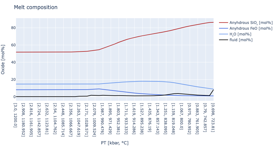

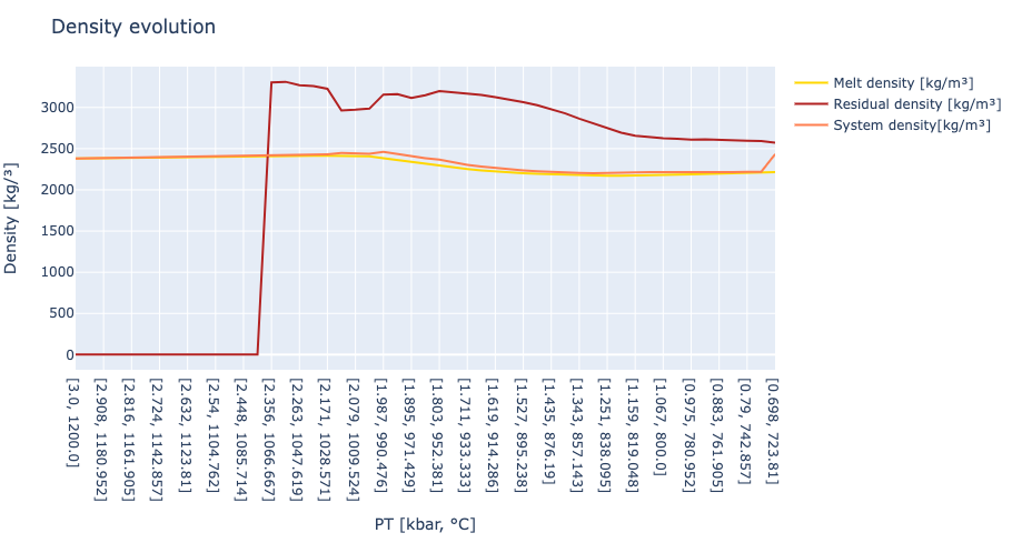
# section to plot density evolution
trace1 = scatter(   x       = x, 
                    y       = melt_density, 
                    name    = "Melt density [kg/m³]",
                    line    = attr( color   = "gold", 
                                    width   = 2)                )
                      
trace2 = scatter(   x       = x, 
                    y       = residual_density, 
                    name    = "Residual density [kg/m³]",
                    line    = attr( color   = "firebrick", 
                                    width   = 2)                )
                      
trace3 = scatter(   x       = x, 
                    y       = system_density, 
                    name    = "System density[kg/m³]",
                    line    = attr( color   = "coral", 
                                    width   = 2)                )

layout = Layout(    title           = "Density evolution",
                    xaxis_title     = "PT [kbar, °C]",
                    yaxis_title     = "Density [kg/³]")


plot([trace1,trace2,trace3], layout)