Introduction to MAGEMin_C

Table of Contents

• Requirements

• Installation & Setup

  • 1. Create the working directory

  • 2. Install packages

• First minimization script

  • 1. Create a new Julia script

  • 2. Load MAGEMin_C and Plots packages

  • 3. Initialize MAGEMin

  • 4. Provide system information

  • 5. Call single point minimization routine

  • 6. Perform the stable phase equilibrium calculation

  • 7. Access minimization results

  • 8. Retrieve garnet composition in wt

  • 9. Plot garnet composition

  • 10. Plot melt and solid bulk composition

• Exercises

  • E.1. Calculate residual composition

Requirements

• This tutorial assumes you have Visual Studio Code and Julia installed.

• Detailed documentation is provided here

Installation & Setup

Create a dedicated local folder for MAGEMin_C to live in its own environment. This avoids potential conflicts with other packages such as MAGEMinApp.

1. Create the working directory

cd /where_you_want_your_folder
mkdir 2026_Beijing_MAGEMin
cd 2026_Beijing_MAGEMin
julia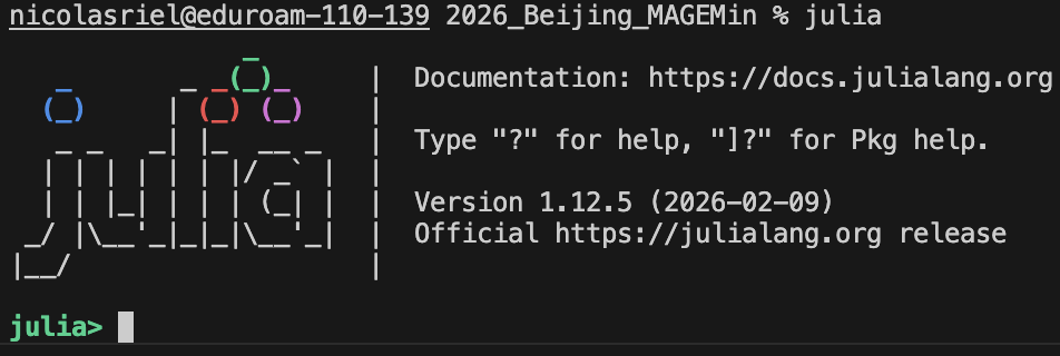

2. Install packages

Open the Julia package manager by pressing ], then activate the local environment and add the required packages:

] 
activate .
add MAGEMin_C, Plots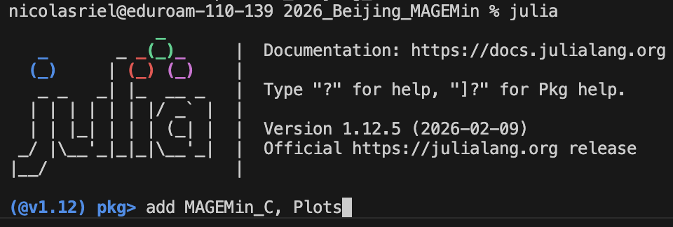

This installs both MAGEMin_C and Plots, the latter being the visualization package used throughout this tutorial. More advanced alternatives such as Makie or PlotlyJS exist but are beyond the scope of this introduction.

Note

activate . creates a local Julia environment in 2026_Beijing_MAGEMin/ where MAGEMin_C and Plots are installed. If you close the terminal, you will need to re-activate it (] activate .) to reload the local environment.

First minimization script

1. Create a new Julia script

Simply open a new terminal in the 2026_Beijing_MAGEMin folder and type:

code first_minimization.jl

This creates a Julia script (.jl) and opens the file in VS Code.

2. Load MAGEMin_C and Plots packages

In the empty file, add the following line at the top of the file:

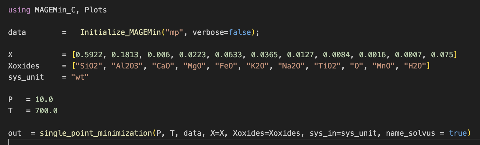
using MAGEMin_C, Plots

3. Initialize MAGEMin

data        =   Initialize_MAGEMin("mp", verbose=false);

This command initializes MAGEMin using the "mp" database (or a-x set of models) which stands for "metapelite" (White et al., 2014).

Available thermodynamic a-x sets:

Acronym	Dataset	Reference
mtl	Mantle	Holland et al., 2013
mp	Metapelite	White et al., 2014
mb	Metabasite	Green et al., 2016
ig	Igneous	Green et al., 2025 (updated from Holland et al., 2018)
igad	Igneous alkaline dry	Weller et al., 2024
um	Ultramafic	Evans & Frost, 2021
sb11	Stixrude & Lithgow-Bertelloni	2011
sb21	Stixrude & Lithgow-Bertelloni	2021
sb24	Stixrude & Lithgow-Bertelloni	2024
ume	Ultramafic extended	Green et al., 2016 + Evans & Frost, 2021
mpe	Extended metapelite	White et al., 2014 + Green et al., 2016 + Franzolin et al., 2011 + Diener et al., 2007
mbe	Extended metabasite	Green et al., 2016 + Diener et al., 2007 + Rebay et al., 2022

4. Provide system information

Provide a composition and a system unit:

X           = [0.5922, 0.1813, 0.006, 0.0223, 0.0633, 0.0365, 0.0127, 0.0084, 0.0016, 0.0007, 0.075]
Xoxides     = ["SiO2", "Al2O3", "CaO", "MgO", "FeO", "K2O", "Na2O", "TiO2", "O", "MnO", "H2O"]
sys_unit    = "wt"

Here, we use a water oversaturated average pelite composition. Note that sys_unit can be "wt" or "mol".

Define pressure and temperature:

P   = 10.0
T   = 700.0

5. Call single point minimization routine

out  = single_point_minimization(P, T, data, X=X, Xoxides=Xoxides, sys_in=sys_unit, name_solvus = true)

Here, the argument name_solvus automatically tries to correctly name several instances of the same solution model based on their composition. For instance, feldspar can be either plagioclase pl or alkali-feldspar afs.

At this stage, your first MAGEMin script should look like:

6. Perform the stable phase equilibrium calculation

To execute the script, either copy and paste the content of your script in the Julia terminal or type:

include("first_minimization.jl")

This should result in:

julia> include("first_minimization.jl")
Pressure          : 10.0      [kbar]
Temperature       : 700.0    [Celsius]
     Stable phase | Fraction (mol fraction) 
                g   0.07753 
               mu   0.169 
              liq   0.24053 
               bi   0.09972 
              ilm   0.01863 
                q   0.24848 
               ky   0.04752 
               ru   0.00037 
              H2O   0.09822 
     Stable phase | Fraction (wt fraction) 
                g   0.09343 
               mu   0.19963 
              liq   0.20529 
               bi   0.10707 
              ilm   0.02116 
                q   0.27091 
               ky   0.06987 
               ru   0.00054 
              H2O   0.03211 
     Stable phase | Fraction (vol fraction) 
                g   0.0595 
               mu   0.18 
              liq   0.25537 
               bi   0.09142 
              ilm   0.01096 
                q   0.26397 
               ky   0.04914 
               ru   0.00033 
              H2O   0.0893 
Gibbs free energy : -853.149024  (27 iterations; 16.83 ms)
Oxygen fugacity          : -13.512530621551143
Delta QFM                : 2.495598922485575

The quick output shows you a summary of the results of the calculation, providing you with the stable phases and their mol, wt and vol fractions.

7. Access minimization results

The full output of the calculation is saved in the out structure. The different fields can be accessed in the terminal by typing out. and pressing "tab":

out.

which unfolds to:

out.

G_system        Gamma           MAGEMin_ver     M_sys           PP_syms         PP_vec          P_kbar          SS_syms         SS_vec          T_C             V               Vp              Vp_S            Vs              Vs_S            X
aAl2O3          aFeO            aH2O            aMgO            aSiO2           aTiO2           alpha           buffer          buffer_n        bulk            bulkMod         bulkModulus_M   bulkModulus_S   bulk_F          bulk_F_wt       bulk_M
bulk_M_wt       bulk_S          bulk_S_wt       bulk_res_norm   bulk_wt         dQFM            database        dataset         elements        enthalpy        entropy         eta_M           fO2             frac_F          frac_F_vol      frac_F_wt
frac_M          frac_M_vol      frac_M_wt       frac_S          frac_S_vol      frac_S_wt       iter            mSS_vec         n_PP            n_SS            n_mSS           oxides          ph              ph_frac         ph_frac_1at     ph_frac_vol
ph_frac_wt      ph_id           ph_id_db        ph_type         rho             rho_F           rho_M           rho_S           s_cp            shearMod        shearModulus_S  sol_name        status          time_ms

A full description of every variable and array stored in the out structure is provided here. This includes detailed information on how to access the composition of phases in different units (vol, mol, wt, apfu), fraction but also other properties such as heat capacity, density, seismic velocity and melt viscosity (among others).

For instance, stable phases acronyms can be accessed as:

out.ph

9-element Vector{String}:
 "g"
 "mu"
 "liq"
 "bi"
 "ilm"
 "q"
 "ky"
 "ru"
 "H2O"

...and the mole fraction of stable melt can be accessed as:

out.frac_M

0.2405316872497568

while the volume fraction as:

out.frac_M_vol

0.2553733579195757

where "M", stands for melt and can be replaced by "S" solid, and "F" for fluid.

8. Retrieve garnet composition in wt

To extract the composition of garnet, one needs to access the properties of the "g" phase which are stored in out.SS_vec.

• Note that SS_vec is a sub structure of out that stores all the information about the stable solution phases. Instead, the information about the pure phases are accessed in PP_vec sub-structure.

Because SS_vec is an array of structure of size n solution phase, there are several ways to retrieve the index of garnet. For instance, one could look for the index of garnet in out.ph

id_g = findfirst(out.ph .== "g")

1

then access the information of garnet using id_g as:

out.SS_vec[id_g].

Comp                Comp_apfu           Comp_wt             G                   V                   Vp
Vs                  alpha               bulkMod             compVariables       compVariablesNames  cp
deltaG              emChemPot           emComp              emComp_apfu         emComp_wt           emFrac
emFrac_wt           emNames             enthalpy            entropy             f                   rho
shearMod            siteFractions       siteFractionsNames

and its composition in wt as:

out.SS_vec[id_g].Comp_wt

11-element Vector{Float64}:
 0.38117580289882985
 0.2026163965532957
 0.04357834582077847
 0.06089592806492956
 0.3024411056038425
 0.0
 0.0
 0.0
 0.002041744392071351
 0.007250676666252689
 0.0

Warning

The ordering of the output oxides may differ from the input ones. This is because MAGEMin internally reorganizes them. To check the ordering of the oxides in the out structure simply type:

out.oxides

11-element Vector{String}:
 "SiO2"
 "Al2O3"
 "CaO"
 "MgO"
 "FeO"
 "K2O"
 "Na2O"
 "TiO2"
 "O"
 "MnO"
 "H2O"

In a similar manner, the composition in atom per formula unit can be accessed as:

out.SS_vec[id_g].Comp_apfu

which gives:

11-element Vector{Float64}:
  2.9999999999999996
  1.8793194615095314
  0.36744182626293087
  0.7145112355900585
  1.9903978756455607
  0.0
  0.0
  0.0
 12.060340269245234
  0.048329600991918464
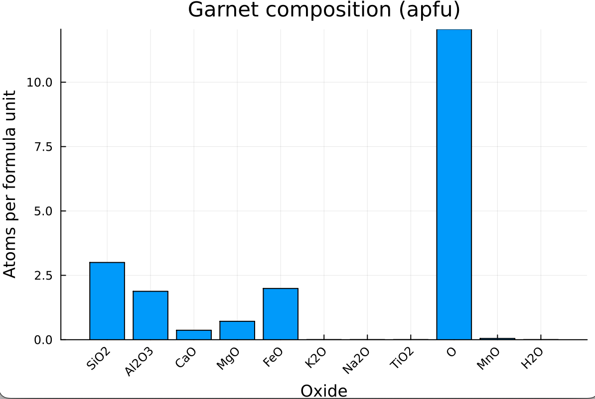
  0.0

9. Plot garnet composition

Using Plots.jl, we can visualize the garnet composition (in apfu) as a bar chart where each bar is labeled by its oxide:

bar(out.oxides, out.SS_vec[id_g].Comp_apfu,
xlabel  = "Oxide",
ylabel  = "Atoms per formula unit",
title   = "Garnet composition (apfu)",
legend  = false,
xrotation = 45)

which should give:

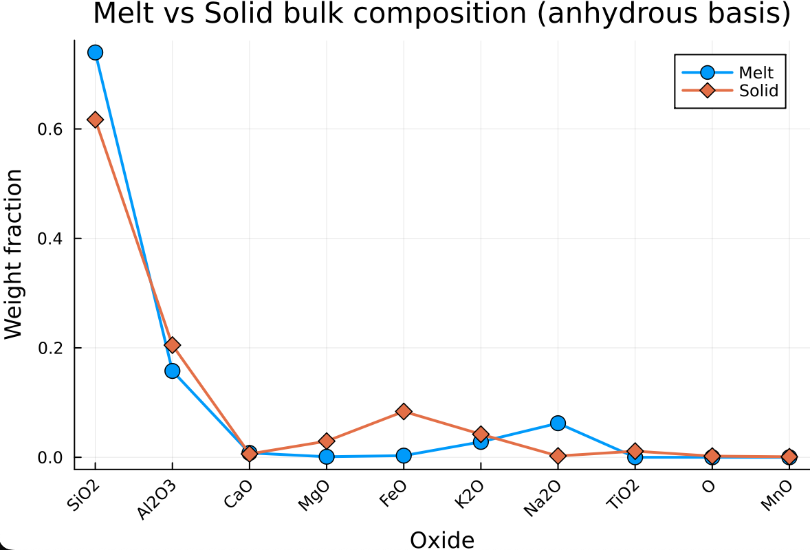
10. Plot melt and solid bulk composition

We can compare the bulk composition of the melt and solid sub-systems on an anhydrous basis using a scatter + line diagram:

first renormalize the composition of the solid and the melt in an anhydrous basis:

dry_oxides      = findall(out.oxides .!= "H2O")
bulk_M_wt_dry   = out.bulk_M_wt[dry_oxides] ./ sum(out.bulk_M_wt[dry_oxides])
bulk_S_wt_dry   = out.bulk_S_wt[dry_oxides] ./ sum(out.bulk_S_wt[dry_oxides])

plot(out.oxides[dry_oxides], bulk_M_wt_dry,
    label       = "Melt",
    markershape = :circle,
    markersize  = 6,
    linewidth   = 2,
    xlabel      = "Oxide",
    ylabel      = "Weight fraction",
    title       = "Melt vs Solid bulk composition (anhydrous basis)",
    xrotation   = 45)

plot!(out.oxides[dry_oxides], bulk_S_wt_dry,
    label       = "Solid",
    markershape = :diamond,
    markersize  = 6,
    linewidth   = 2)

which should give:

Exercises

E.1. Calculate residual composition

• Assuming that any volume of melt > 0.07 vol_fraction is extracted, as well as any free water is extracted, calculate the remaining residual bulk-rock composition in wt fraction.

  • Mind that  

  • Densities of solid, melt and fluid can be accessed as out.rho_S, out.rho_M and out.rho_F

  • Solid, melt and fluid wt compositions can be accessed as out.bulk_S_wt, out.bulk_M_wt and out.bulk_F_wt

• Using the plot from point #10 (Plot melt and solid bulk composition), add the composition of the residual to the plot