Info

• MAGEMinApp.jl Tips

• 1. Phase diagrams tab

  • 1.1 Setup panel

  • 1.2 Bulk-rock composition panel

  • 1.3 Trace-element composition panel

  • 1.4 General parameters panel

• 2. Diagram sub-tab

  • 2.1 Informations panel

  • 2.2 Display options panel

  • 2.3 Isopleths panel

  • 2.4 Draw path panel

  • 2.5 Thermobarometric intersection panel

• 3. Trace-elements sub-tab

  • 3.1 Display options

  • 3.2 TE Isopleths

  • 3.3 Export and save

• 4. PTX path tab

  • 4.1 Bulk-rock composition panel

  • 4.2 Trace Elements panel

  • 4.3 Path options panel

  • 4.4 PTX save and export

• 5. General information tab

• Trace-element Kd models

MAGEMinApp.jl Tips

Tip

• Mind that when performing a calculation progress is indicated either by the progress bar at the top right corner of the interface, or by changing the name of your web-browser tab (where MAGEMinApp is opened) to Updating...

• Once a calculation is launched, avoid performing other actions as it may lead to calculation failure

MAGEMinApp.jl interface

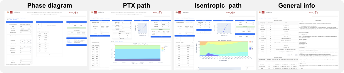
The graphic user interface includes 3 main tabs: two for phase equilibrium calculations and one for supporting reference data.

This tab contains three sub-tabs: Setup (configuration), Diagram (visualization and post-processing) and Trace-elements (trace-element partitioning and accessory phase saturation). It allows you to generate and post-process P-T, T-X, P-X, PT-X and T-T polymetamorphic phase diagrams.

Available thermodynamic databases are presented here. All other options and parameters are detailed below.

---

1. Phase diagrams tab

1.1. Setup panel

Setup

Caption

Thermodynamic database — select among available thermodynamic databases (ig, mp, mb, um, mtl, sb11, sb21, sb24) Dataset — select among available thermodynamic datasets for the chosen database Phase selection — expand to activate or deactivate individual solution and pure phase models Diagram type — P-T, P-X, T-X, PT-X, or T-T (polymetamorphic) Solidus H₂O-saturated — saturate the first melt in water at the solidus (true/false) Additional H₂O [mol%] — amount of extra H₂O added when solidus saturation is active (0–100) Clinopyroxene — switch between Omphacite (Omph) and Augite (Aug) for the metabasite database Limit Ca-opx — enforce a maximum Ca content in orthopyroxene (0–1; default 0.5) TE predictive model — enable trace-element partitioning at suprasolidus conditions (true/false) KD model — lattice-strain Kd database: OL (O. Laurent, 2012) or CO (J. Cornet, 2019) Zr saturation — zircon saturation model: none, WH (Watson & Harrison, 1983), B (Boehnke et al., 2013), CB (Crisp & Berry, 2022) P₂O₅ saturation — fluorapatite saturation model: none, Klein26, Tollari06, HWBea92 S saturation — sulfide saturation model: none, Liu07, Oneill21 CO₂ saturation — CO₂ fluid saturation model: none, SY26 (Sun & Yao, 2026) EODC — empirical oxide–distribution coefficient model: KP, IL, B, AV; with an associated ratio field (0–1) Upload Kd's — drag-and-drop zone to load a custom Kd database file Pressure [kbar] — minimum and maximum pressure range for the diagram Temperature [°C] — minimum and maximum temperature range for the diagram Fixed pressure / temperature — single pressure or temperature value for P-X and T-X diagram types Initial grid subdivision — sets the starting grid resolution (2–9; default 4, yielding a 16×16 grid) Refinement type — refine on phase boundaries (ph) or dominant end-members (em) Refinement levels — number of adaptive mesh refinement levels applied (default 3) Boost mode — use the previous refinement level as an initial guess for the next (true/false) Buffer — oxygen fugacity buffer or fixed oxide activity: none, QFM, MW, IW, QIF, CCO, HM, NNO, aH₂O, aO₂, aFeO, aMgO, aAl₂O₃, aTiO₂ Solver — Gibbs energy minimization algorithm: pge (projected gradient), lp (linear programming), hyb (hybrid) Verbose — level of output in the Julia terminal: -1 (none), 0 (light), 1 (full) Seismic averaging — averaging scheme for seismic velocities: 0 (VRH – Voigt-Reuss-Hill), 1 (HS – Hashin-Shtrikman) Weight factor — mixing weight between Voigt and Reuss bounds (0–1; default 0.5) Specific Cp — 0: G₀ (no latent heat); 1: G_system (includes latent heat of reaction)

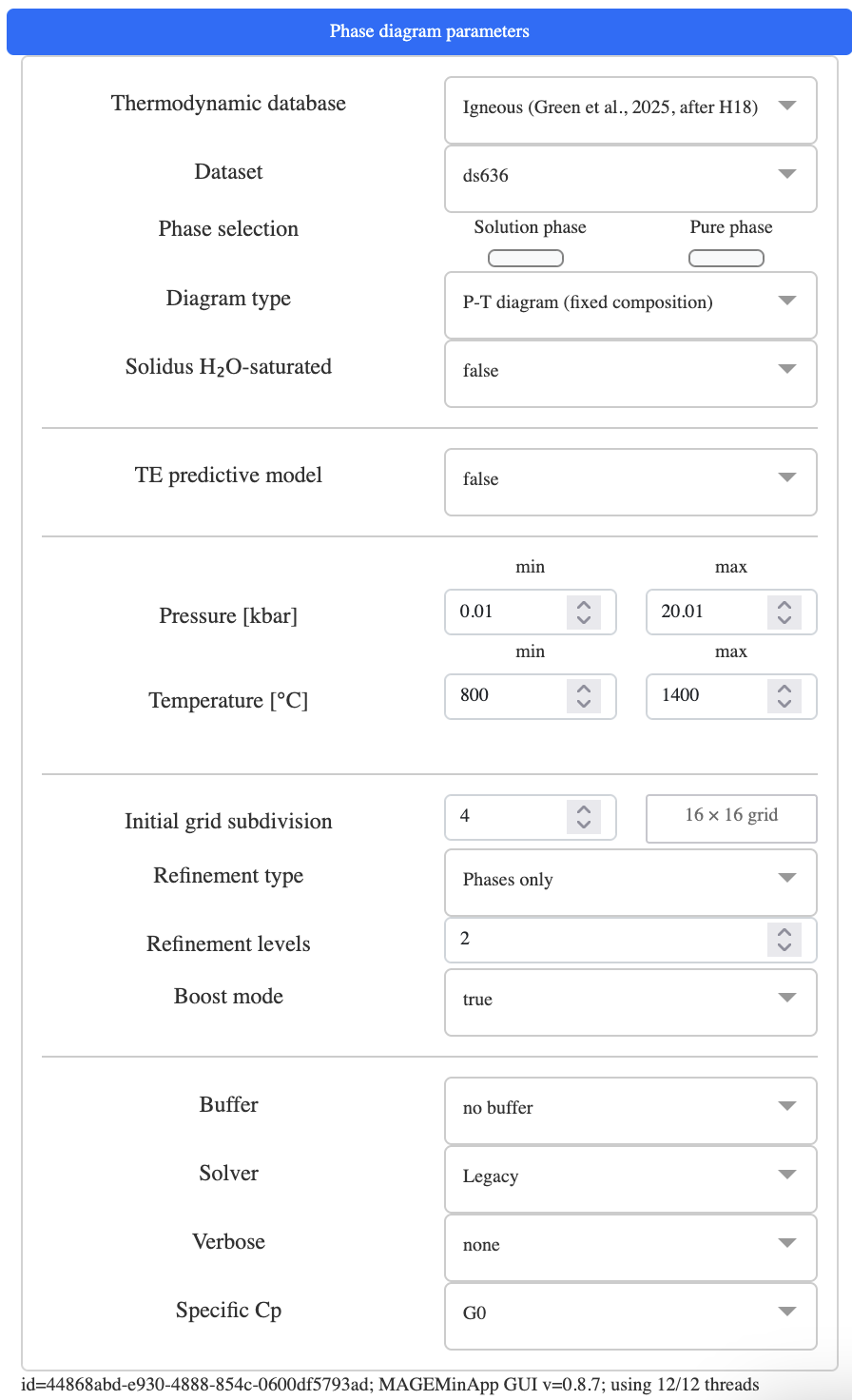1.2. Bulk-rock composition panel

Setup

Caption

System unit — display and input the bulk-rock composition in mol% or wt% Drag and drop — upload a bulk-rock CSV file or drag and drop it onto the dashed upload zone Bulk-rock list — select from pre-defined or previously uploaded bulk-rock compositions Composition table — editable table showing the loaded oxide composition; values can be modified directly Buffer offset — shift the oxygen fugacity relative to the selected buffer (–50 to +50; default 0)

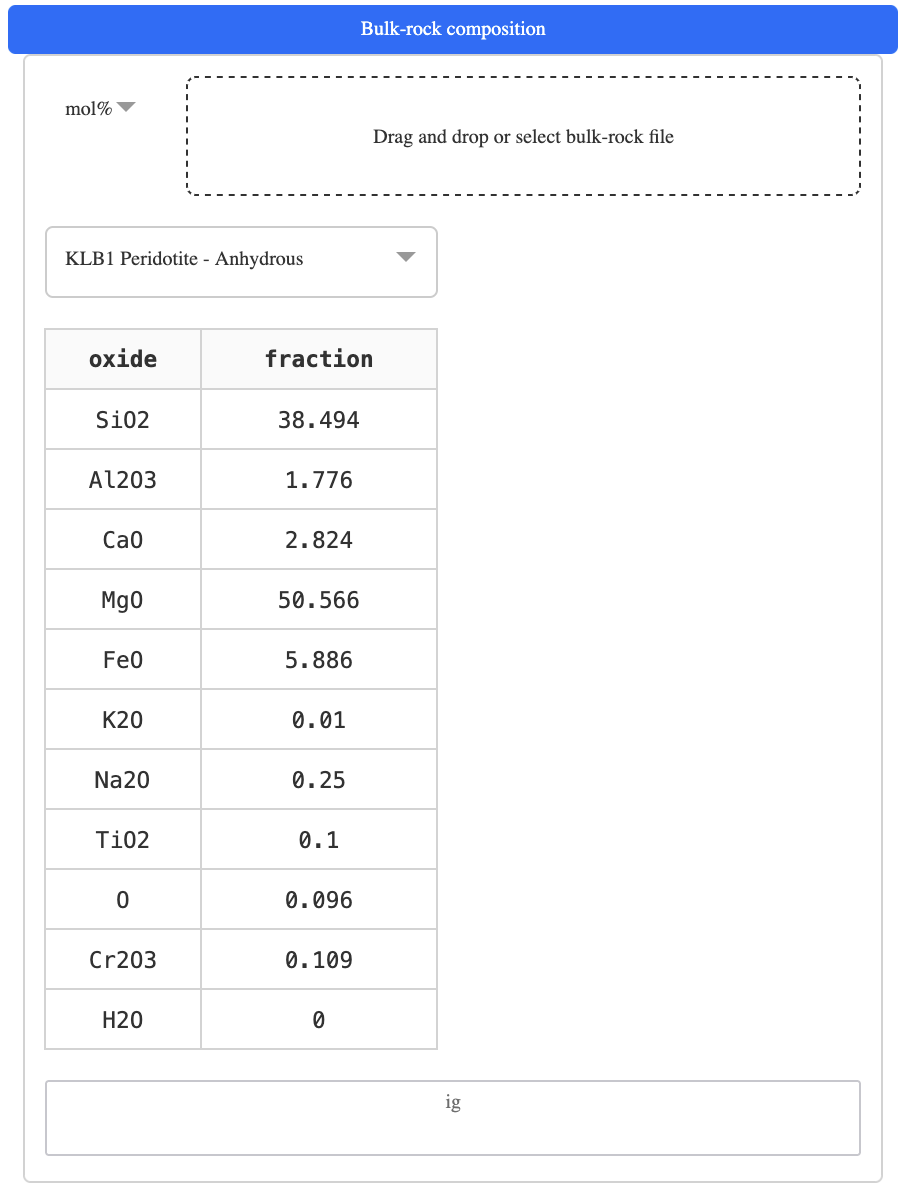1.3. Trace-element composition panel

When TE predictive model = true, a third collapsible panel appears below the bulk-rock panel:

Trace-element panel	Caption
	Drag and drop — upload a custom trace-element file (CSV with element and μg/g columns) TE composition list — select from built-in trace-element compositions TE table — editable table showing element concentrations in μg/g (ppm)

1.4. General parameters panel

General parameters

Caption

Title — set the title for the phase diagram; use Update/Reset buttons to apply or revert Compute phase diagram — launch the calculation (green button) Save/Load diagram — save or reload a computed diagram together with all selected options (modal dialogs with filename input) Advanced options — load custom W interaction parameters from a file path Directory window — read-only field showing the folder where exported CSV data will be saved Help and contact — links to post issues and request support Contributors — list of people who contributed to MAGEMinApp

---

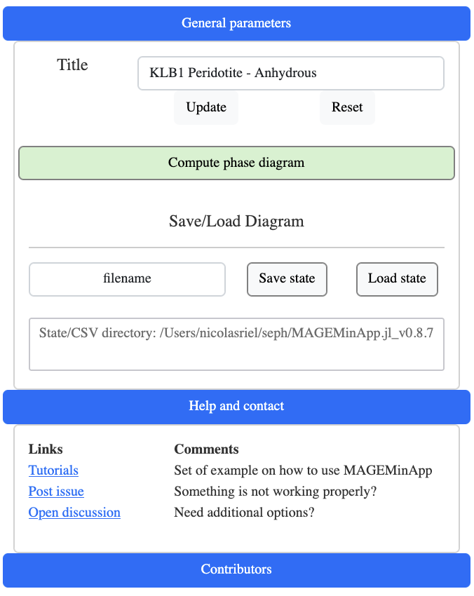2. Diagram sub-tab

The Diagram sub-tab has a right-hand sidebar with five tabs: Informations, Display options, Isopleths, Draw path, and Thermobarometric intersection.

2.1. Informations panel

Informations

Caption

Computation info — read-only summary of the last computed point (phase assemblage, conditions, fractions) Pie unit — unit for the pie chart: mol%, wt%, or vol% Pie chart — shows the modal fractions of stable phases at the selected point Transfer point as bulk — transfer the composition of Solid, Melt, or Whole-rock at the selected point to the bulk-rock composition panel; provide a name and click Transfer Mineral composition table — oxide composition of each stable phase at the clicked point in mol%, wt%, and apfu (read-only, copyable) Save point — save the full point information to a CSV or text file Save all — save all computed points to a CSV file Export references — export citations for the active models as a BibTeX file Code availability — display a ready-to-use statement for methods sections MAGEMin_C snippet — show the equivalent MAGEMin_C.jl code to reproduce the selected point calculation

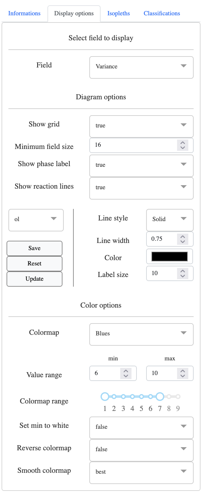
2.2. Display options panel

Display options

Caption

Field — select the scalar field to display as a color map. Available fields: Phase topology: Hash, Variance, #Phases Thermodynamics: G_system, entropy, enthalpy, s_cp, alpha, Specific_Cp Fugacities and activities: fO2, dQFM, aH2O, aFeO, aMgO, aAl2O3, aSiO2, aTiO2 Physical properties: eta_M, rho, rho_S, rho_M, Delta_rho Melt/solid fractions: frac_S, frac_S_wt, frac_S_vol, frac_M, frac_M_wt, frac_M_vol Seismic velocities: Vp, Vs, Vp_S, Vs_S, Vp/Vs, Vp_S/Vs_S Diagnostics: bulk_res_norm, time_ms, status Show grid — display the adaptive mesh refinement grid (true/false) Minimum field size — minimum number of cells for a field to receive a phase label (0–1024; default 16) Show phase label — show or hide phase assemblage labels Show reaction lines — show or hide phase boundary lines Reaction line customization — change the style (solid, dot, dash, longdash, dashdot, longdashdot), width (0–10 px), color and label size of individual reaction lines; Save/Reset/Update buttons apply the changes Modify phase colors — open a color editor for each stable phase; colors persist after recalculation when saved Colormap — choose among: blackbody, Blues, cividis, Greens, Greys, hot, jet, RdBu, Reds, viridis, YlGnBu, YlOrRd Value range — manual min/max for the color scale Colormap range — slider restricting which portion of the colormap is used (1–9) Set min to white — set the minimum value of the field to white (incompatible with Colormap range) Reverse colormap — invert the colormap direction Smooth colormap — interpolation quality: fast, best, or none

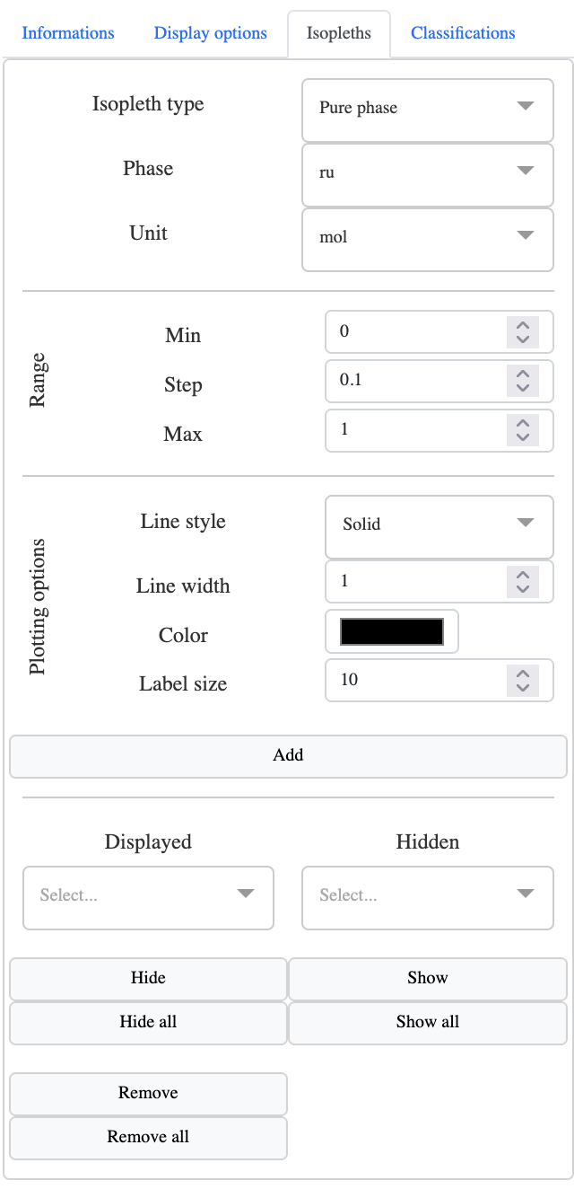
2.3. Isopleths panel

Isopleths

Caption

Isopleth type — pure phase (pp), solution phase (ss), or other (of) Phase — select the phase to contour (depends on isopleth type) Field — for "other" type: mode, oxide composition, end-member mode, Mg#, or custom calculator (apfu, oxides, site fractions) Remove excess fluid — exclude fluid from the normalization when computing fractions (true/false) Unit — mol, wt, or vol Custom calculator — enter an expression (e.g., FeO/(MgO+FeO)) using oxide names or site fractions Range: min / step / max — define the isocontour interval Line style — solid, dot, dash, longdash, dashdot, longdashdot Line width — line thickness in pixels (0–10) Color — color picker for the isocontour lines Label size — font size for isocontour labels (6–20) Add — add the configured isocontour to the diagram Displayed / Hidden lists — manage which isopleths are currently shown or hidden Hide / Hide all / Show / Show all / Remove / Remove all — batch management buttons

2.4. Draw path panel

This panel allows you to manually trace a P-T path directly on the phase diagram by clicking points, then extract the phase evolution along it.

Draw path

Caption

Record — toggle on to start recording clicked points on the diagram as path nodes Point counter — displays the number of recorded points Clear — remove all recorded points Remove last — delete the most recently added point System unit — unit for the generated path data: mol, wt, or vol Generate — compute the phase fractions and compositions along the recorded P-T path Path table — read-only table showing the recorded path points (#, P [kbar], T [°C]) Phase fractions plot — area chart of stable phase fractions along the generated path (expandable)

2.5. Thermobarometric intersection panel

This panel adds isopleths derived from measured mineral compositions to the diagram and finds their intersection to estimate P-T conditions.

Thermobarometric intersection

Caption

Upload CSV — drag-and-drop a CSV file containing measured mineral compositions Phase — select the mineral phase from those available in the uploaded data Refresh phases — reload the phase list after uploading a new file Color — choose the color for the intersection isopleths Composition unit — unit for the input data: wt, mol, or apfu Formula input — enter an oxide or end-member expression to convert to a contourable field (e.g., FeO/(MgO+FeO)) Add formula — register the expression for contouring Formula table — list of registered formulas (#, phase, formula) Remove last / Remove all — manage the formula list Generate — compute and overlay the isopleths on the phase diagram Intersection plot — shows the overlapping isopleths with a statistics table summarizing the estimated P-T conditions (expandable)

---

3. Trace-elements sub-tab

The Trace-elements sub-tab becomes active after a phase diagram has been computed with TE predictive model = true. It displays element distributions and saturation fields across the phase diagram.

3.1. Display options

TE Display options

Caption

Field type — choose the category of field to display: Zircon, Sulfide, Fluorapatite, CO₂ saturation, Trace element Field — specific variable within the selected field type: Zircon: Sat_Zr_liq [ppm], zrc_wt [wt fraction] Sulfide: Sat_S_liq [ppm], sulf_wt [wt fraction] Fluorapatite: Sat_P2O5_liq [ppm], fapt_wt [wt fraction] CO₂ saturation: Sat_CO2_liq [ppm], fl_CO2_wt [wt fraction] Trace element: concentration in the melt via Field builder Field builder (Trace element only) — enter a custom expression using [M_X] for element X in the melt (e.g., [M_Dy] / [M_Yb]); set normalization (none, bulk, chondrite) and click Compute and display Available phases — list of phases for which TE concentrations are available Colormap — same options as the phase diagram colormap Value range — manual color scale min/max Colormap range — slider restricting the colormap portion used Set min to white / Reverse / Smooth — same as in the phase diagram Display options

3.2. TE Isopleths

The Isopleths panel in the Trace-elements sub-tab works identically to the one in the Diagram sub-tab but operates on TE and saturation fields (Zircon, Sulfide, Fluorapatite, CO₂ saturation, Trace element) instead of thermodynamic fields.

3.3. Export and save

• Export figure — save the current TE diagram as an image file

• Export all layers — save each TE field layer as a separate image

• Save point (csv) — save the TE data at the clicked point to CSV

• Save all (csv) — save TE data for all computed points to CSV

• Export references (bibtex) — export BibTeX citations for the active Kd and saturation models

---

4. PTX path tab

The PTX path tab is divided into a left configuration panel and a central results area. It supports all P-T-X path modes from the same interface, including isentropic paths (previously a separate tab; merged in v1.2.1).

4.1. Bulk-rock composition panel

Same controls as the phase diagram bulk-rock panel (§1.2). When Assimilation = true, a second bulk-rock composition panel appears for the assimilated end-member.

4.2. Trace Elements panel

Appears when TE predictive model = true in Path options.

Trace Elements (PTX)

Caption

KD model — lattice-strain Kd database: OL (O. Laurent, 2012) or CO (J. Cornet, 2019) Zr saturation — none, Watson 1979 (WH), or Blundy 2022 (CB) S saturation — none or Liu 2021 (Liu07) P₂O₅ saturation — none or Tollari 2006 CO₂ saturation — none or SY26 (Sun & Yao, 2026) Upload trace-element file — drag-and-drop a CSV file with element concentrations Initial TE bulk composition [μg/g] — editable table with element concentrations; pre-populate from built-in database dropdown Assimilant TE bulk composition [μg/g] — second TE table for the assimilated end-member (visible when Assimilation = true)

4.3. Path options panel

Path options

Caption

Resolution — number of calculation steps between two consecutive path points (1–1024; default 32) P-T-X mode — Equilibrium, Fractional melting, or Fractional crystallization Assimilation — enable progressive addition of a second bulk-rock composition (true/false) TE predictive model — enable trace-element partitioning along the path (true/false) Connectivity threshold [%] — melt fraction above which melt is extracted during fractional melting (0–100; default 7); only visible in fractional melting mode Residual rock fraction [%] — fraction of solid entrained by the fractionating melt during fractional crystallization (0–100; default 0); only visible in fractional crystallization mode Isentropic — compute an isentropic (constant-entropy) path using bisection on temperature (true/false) Solidus H₂O-saturated — saturate the first melt in water at the solidus (true/false) Additional H₂O [mol%] — extra H₂O added at water saturation (visible when Solidus H₂O-saturated = true) Compute path — launch the P-T-X path calculation (green button)

4.4. PTX save and export

All export options are located in the Path options panel:

Button	Content
Save path → csv	Full path: P, T, phase fractions and compositions at each step
Save path → csv line	Same but all steps on a single row
Save cumulate → csv file	Composition of the cumulate (extracted solid) at each step
Save trace elements → csv file	TE concentrations in melt, solid and minerals at each step (requires TE computation)
Save cumulate TE → csv file	Integrated cumulate TE composition at each step (requires TE computation)
Export references → bibtex file	BibTeX citations for active models and database

Note

• The Save trace elements and Save cumulate TE buttons are only active after trace elements have been computed.

• The export path is printed in the Julia terminal.

---

5. General information tab

Provides static reference data across three sections:

• Solution phases table — name, abbreviation, and solvus flag for all solution phases in the selected database (filterable, 16 rows per page)

• End-members table — end-member name, abbreviation, and stoichiometric formula (filterable, 16 rows per page)

• CSV bulk-rock format — example table showing the required column structure for bulk-rock input files (title, comments, db, sysUnit, oxide columns, optional _frac2 variants)

• Trace-element Kd tables — three tabs subdivided by SiO₂ content of the melt (SiO2 < 52 wt%, 52 ≤ SiO2 < 63 wt%, 63 wt% ≤ SiO2); each shows the element × mineral Kd matrix (filterable, 32 rows per page)

• Calculation details — expandable cards describing phase deactivation logic, oxide activity formulation, water saturation methodology, specific heat capacity calculation, and the site fraction calculator

---

Note

Trace-element partitioning model descriptions and Kd tables are documented in the Thermodynamic Databases page.