MAGEMin_C fractional melting
Table of Contents
Now that we have introduced how to perform iterative calculations, we can dynamically update the active bulk-rock composition during the iterations.
Fractional melting
1. Create a new script
code MAGEMin_C_fractional_melting.jl2. Load and initialize
Like previously, let's load the necessary packages, initialize MAGEMin using the metapelite "mp" database, and define a similar pressure and temperature range:
using MAGEMin_C, Plots, ProgressMeter

data        =   Initialize_MAGEMin("mp", verbose=false);

X           = [0.5922, 0.1813, 0.006, 0.0223, 0.0633, 0.0365, 0.0127, 0.0084, 0.0016, 0.0007, 0.075]
Xoxides     = ["SiO2", "Al2O3", "CaO", "MgO", "FeO", "K2O", "Na2O", "TiO2", "O", "MnO", "H2O"]
sys_unit    = "wt"

P           = 1.0
T_step      = 2.0
T           = [600:T_step:1000;]

n_calc      = length(T)
Out_XY      = Vector{out_struct}(undef,n_calc)
We can then define the connectivity threshold using the standard 7.0 vol% value (Rosenberg & Handy, 2005):
MCT = 0.07As in the first example, this value will be used to recompute the bulk-rock composition while keeping only MCT vol fraction of melt.
3. Fractional melting
Let's now modify the calculation loop to update the bulk-rock composition dynamically by extracting any melt volume > MCT:
residual_comp_wt = copy(X)
@showprogress for i in 1:n_calc
    Out_XY[i]           = single_point_minimization(P, T[i], data, X=residual_comp_wt, Xoxides=Xoxides, sys_in=sys_unit, name_solvus = true, scp=1)

    if Out_XY[i].frac_M_vol .> MCT
        residual_comp_wt    = Out_XY[i].rho_M * MCT  .* Out_XY[i].bulk_M_wt .+ Out_XY[i].rho_S * Out_XY[i].frac_S_vol .* Out_XY[i].bulk_S_wt
    else
        residual_comp_wt    = Out_XY[i].rho_M * Out_XY[i].frac_M_vol  .* Out_XY[i].bulk_M_wt .+ Out_XY[i].rho_S * Out_XY[i].frac_S_vol .* Out_XY[i].bulk_S_wt
    end
    Xoxides             = Out_XY[i].oxides #here we make sure we have the right oxides order!
end
Here, we first make a copy of the starting bulk-rock composition residual_comp_wt = copy(X). The residual_comp_wt is subsequently updated during the iteration as
if Out_XY[i].frac_M_vol .> MCT
    residual_comp_wt    = Out_XY[i].rho_M * MCT  .* Out_XY[i].bulk_M_wt .+ Out_XY[i].rho_S * Out_XY[i].frac_S_vol .* Out_XY[i].bulk_S_wt
else
    residual_comp_wt    = Out_XY[i].rho_M * Out_XY[i].frac_M_vol  .* Out_XY[i].bulk_M_wt .+ Out_XY[i].rho_S * Out_XY[i].frac_S_vol .* Out_XY[i].bulk_S_wt
end
The "if, else" statement allows updating the residual bulk-rock composition when the MCT is reached. Note that we don't renormalize here — this is done internally within MAGEMin.
4. Display melt volume fraction evolution
The evolution of the volume fraction of melt can be visualized using:
melt_vol = [Out_XY[i].frac_M_vol for i=1:n_calc]

plot(T, melt_vol,
    xlabel      = "Temperature [°C]",
    ylabel      = "Fraction [vol]",
    title       = "Batch melting at P = $(P) kbar",
    label       = "Melt",
    linewidth   = 2,
    legend      = :topleft)
which gives:
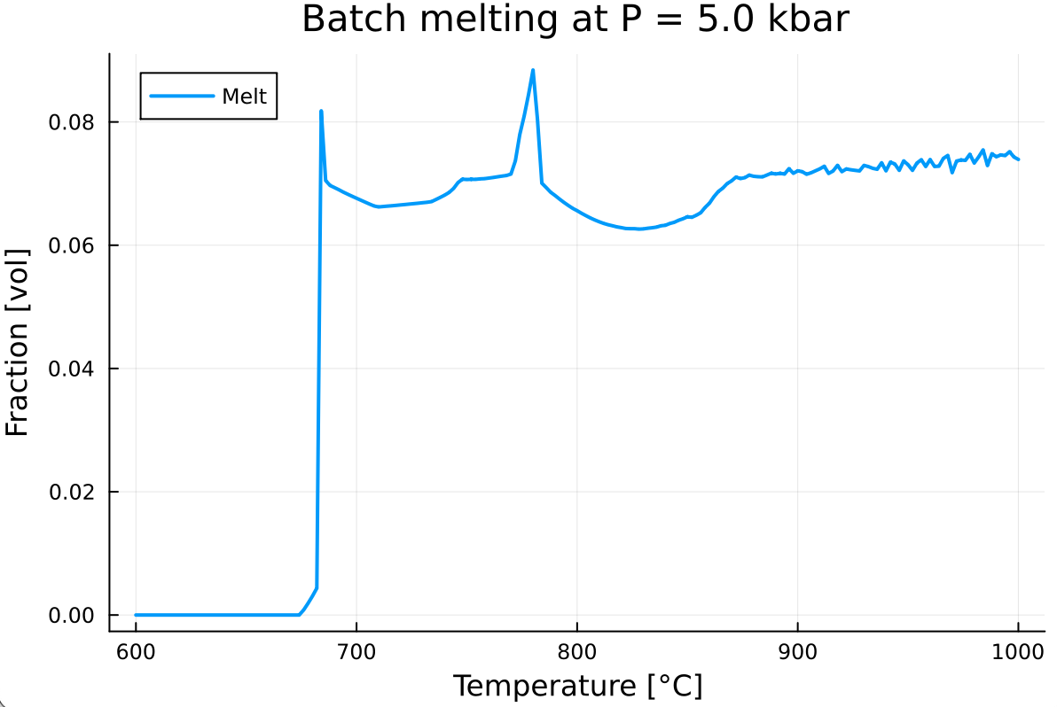
- Notice how the calculated melt volume fraction can spike above the MCT. This is because we visualize the equilibrium melt volume fraction, before extraction.
5. Tracking the evolution of the system mass
While the previous example allows tracking the evolution of the composition of the liquid and solid, it does not properly handle the evolution of the system mass as melt is being removed.
M_system         = 1.0                      # track mass relative to original
extracted_M_wt   = zeros(Float64, n_calc)
M_system_evol    = zeros(Float64, n_calc)

residual_comp_wt = copy(X)
@showprogress for i in 1:n_calc
    Out_XY[i] = single_point_minimization(P, T[i], data, X=residual_comp_wt, Xoxides=Xoxides, sys_in=sys_unit, name_solvus = true, scp=1)

    # mass per unit volume of each sub-system
    m_M     = Out_XY[i].rho_M * Out_XY[i].frac_M_vol
    m_S     = Out_XY[i].rho_S * Out_XY[i].frac_S_vol
    m_total = m_M + m_S

    if Out_XY[i].frac_M_vol > MCT
        m_M_retained     = Out_XY[i].rho_M * MCT
        m_extracted      = Out_XY[i].rho_M * (Out_XY[i].frac_M_vol - MCT)

        # extracted melt as fraction of original system mass
        extracted_M_wt[i] = (m_extracted / m_total) * M_system

        # update remaining system mass
        M_system -= extracted_M_wt[i]

        # residual = retained melt + solid
        residual_comp_wt = m_M_retained .* Out_XY[i].bulk_M_wt .+ m_S .* Out_XY[i].bulk_S_wt
    else
        residual_comp_wt = m_M .* Out_XY[i].bulk_M_wt .+ m_S .* Out_XY[i].bulk_S_wt
    end

    M_system_evol[i] = M_system
    Xoxides          = Out_XY[i].oxides
end
Here, the sub-system masses for both melt and solid are calculated as
The extracted melt mass (wt) is normalized by the total mass (
m_total) of the iteration and the system mass (M_system)The evolutions of both extracted melt mass and system mass are saved in
extracted_M_wtandM_system_evol, respectively
Exercises
E.1. Visualize the results
- First plot the system mass evolution as well the extracted melt mass
- Note that
extracted_M_wtneeds to be converted to a cumulative sum:
- Note that
accumulated_extracted_M_wt = cumsum(extracted_M_wt)This should give: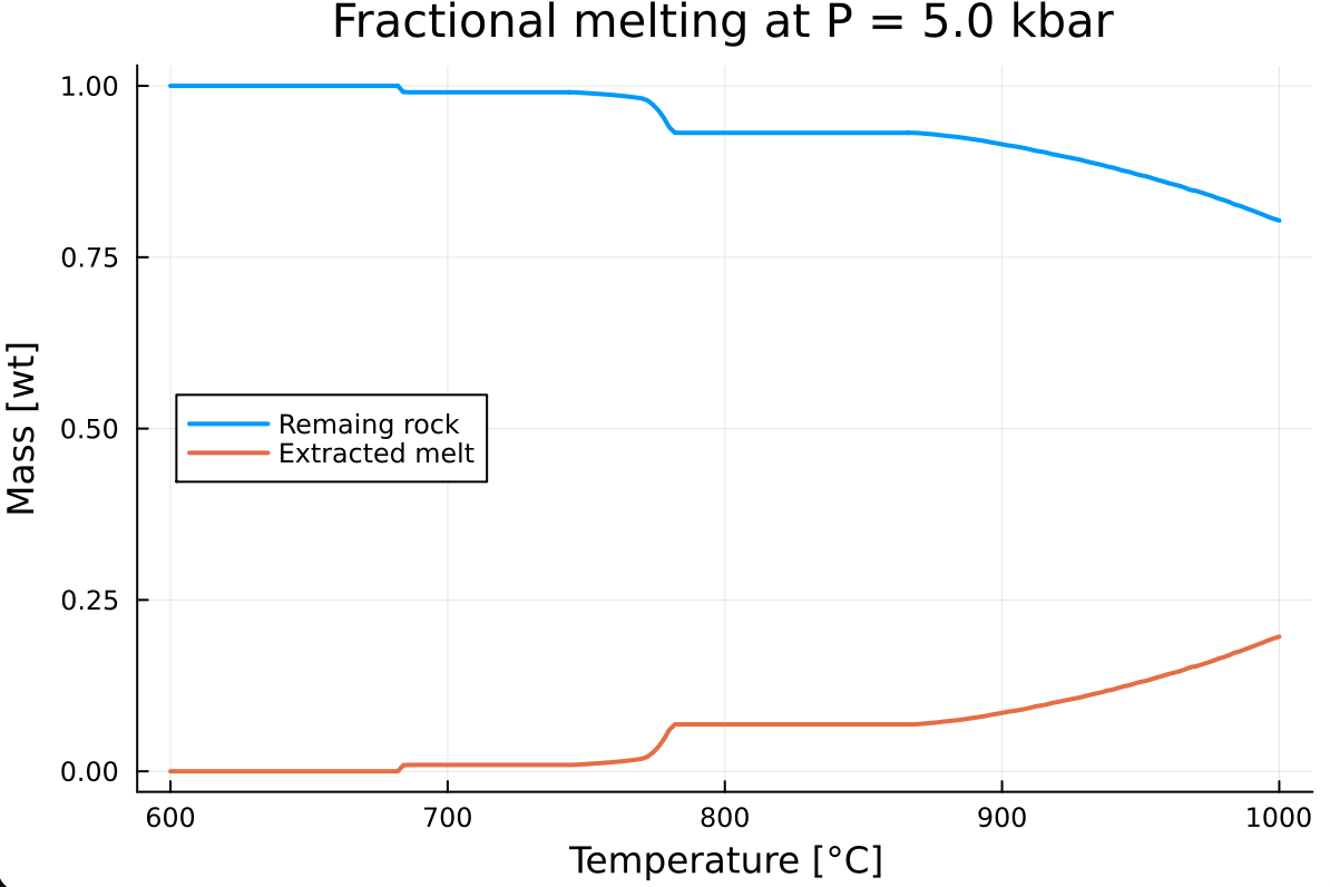
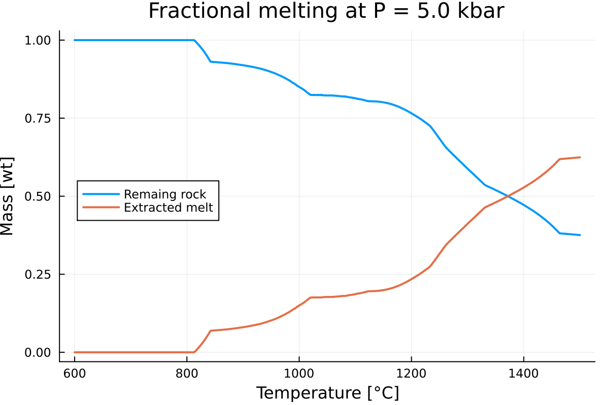
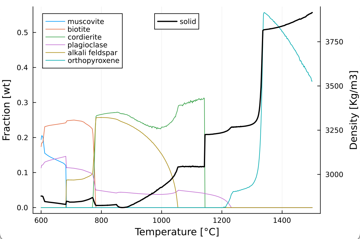
Perform the fractional melting calculation up to 1500°C
Plot the evolution of the wt fraction for key minerals such as muscovite, biotite, cordierite, plagioclase, alkali-feldspar, and orthopyroxene (
mu,bi,cd,pl,afs, andopx).- Create a function to avoid copying and pasting the same code block several times!
Add a twin plot (secondary y-axis) depicting the density of the solid
- Now change the melt connectivity threshold from 0.07 to 0.0. How does that change the results?
- How do you explain the difference?
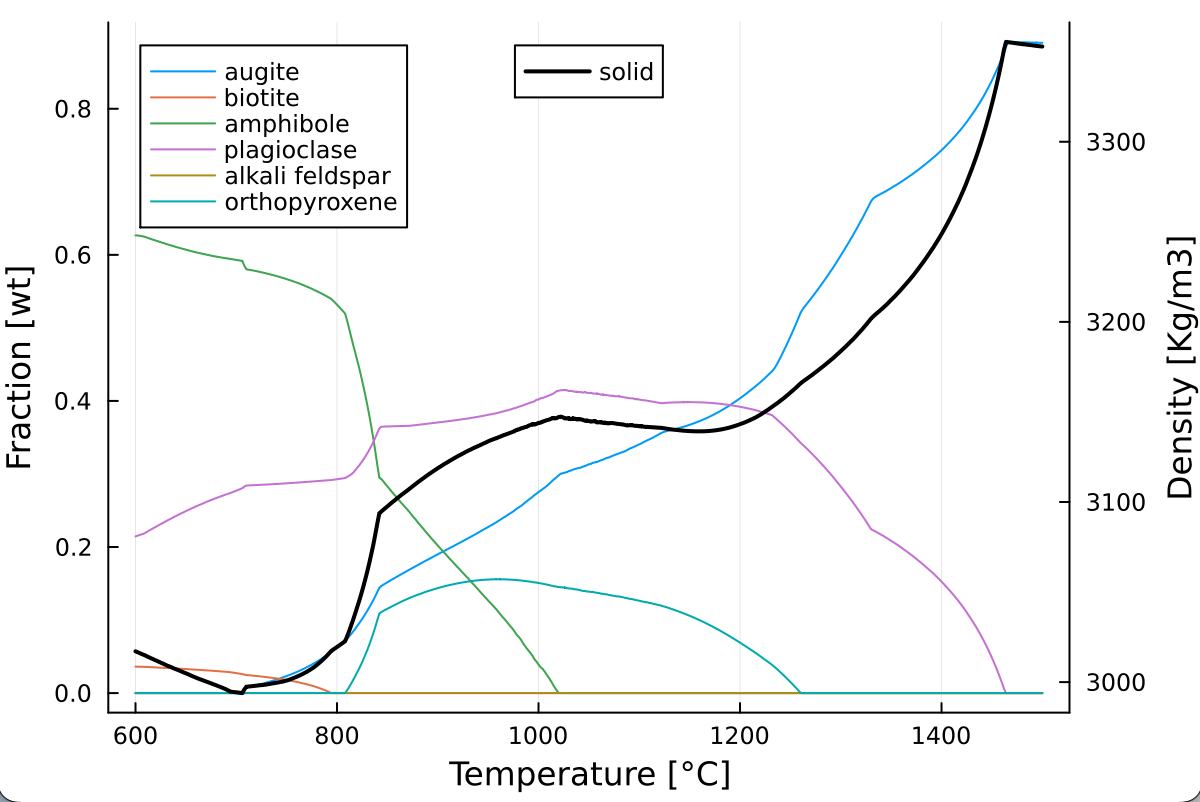
E.2. Fractional melting using metabasite database
Adapt previous script to perform the fractional melting of a metabasite using the metabasite
mbdatabaseuse the world median metabasite composition (Forshaw et al., 2024)
    Xoxides = ["SiO2","Al2O3","CaO","MgO","FeO","K2O","Na2O","TiO2","O","H2O"]
X = [50.7870, 15.3030, 9.4917, 6.7515, 11.3462, 0.4942, 2.7868, 1.3137, 0.3285, 1.4210]- Don't forget to change how MAGEMin is initialized:
data = Initialize_MAGEMin("mb", verbose=false);- Perform the calculation and change the mineral evolution plot to augite, biotite, plagioclase, amphibole alkali-feldspar and orthopyroxene (
aug,pl,amp,afsandopx). This should give: