Phase diagrams tutorials (MAGEMinApp v0.8.6)
Here we provide a set of tutorials to generate various kind of phase diagrams, compute trace-element partitioning and Zr saturation, post-process the results, display various fields, reaction lines and iso-contours, and, export data and save the diagrams as svg graphic vector files.
Info
1. First phase diagram
For the first diagram, simply launch MAGEMinApp and navigate to the Setup sub-tab of the Phase diagram tab. Then click on Compute phase diagram. 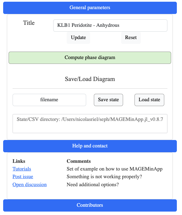
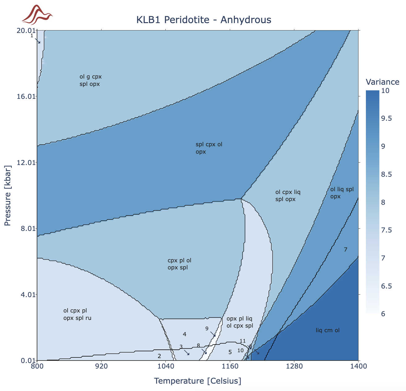
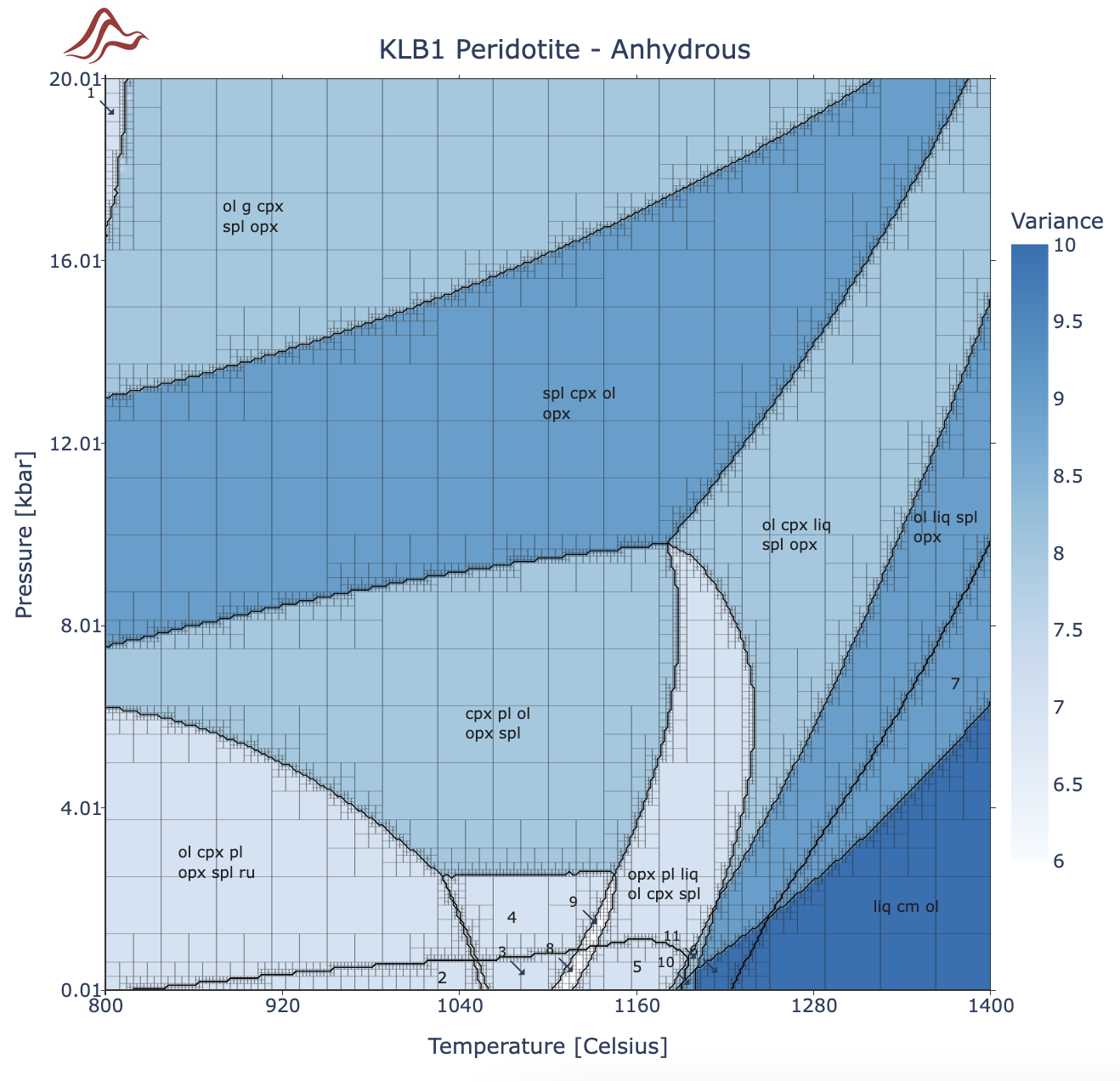
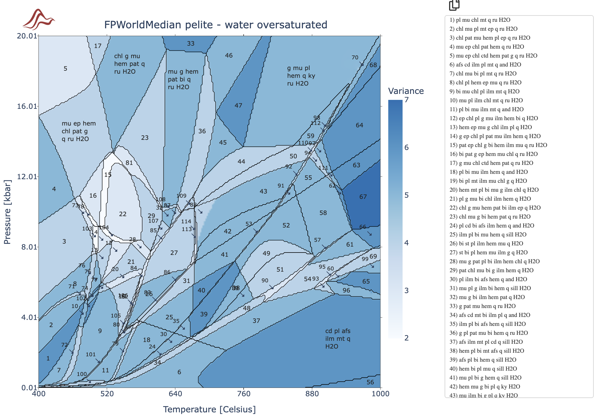
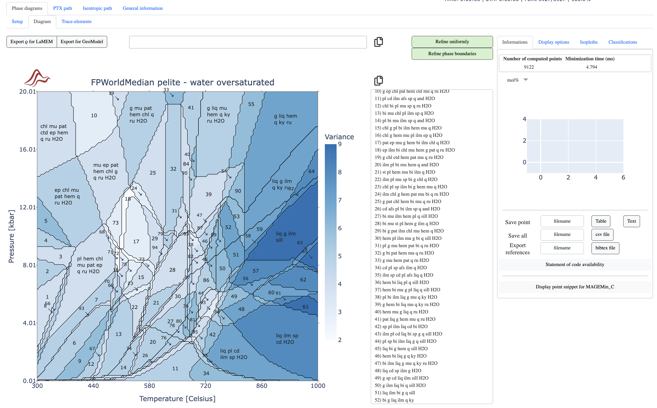
In less than one minute you should get the following result (tab Diagram):
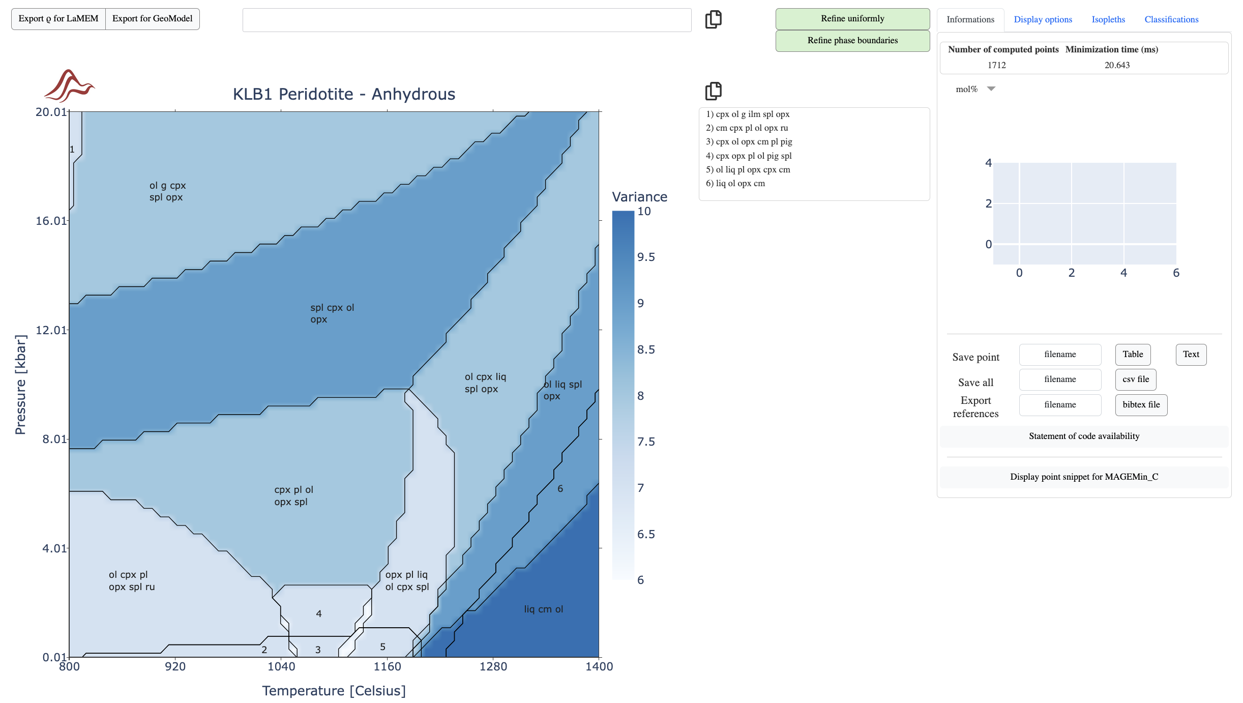
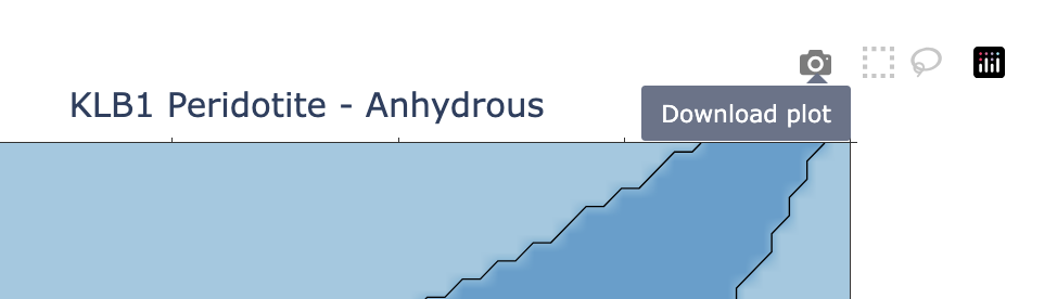
The default field to be displayed is variance. Superimposed on it are the reactions lines (in black) and the phase assemblage labels with a list of labels shown on the right in the event the field size are too small. If you scroll down below the figure you can see the informations about the computation:
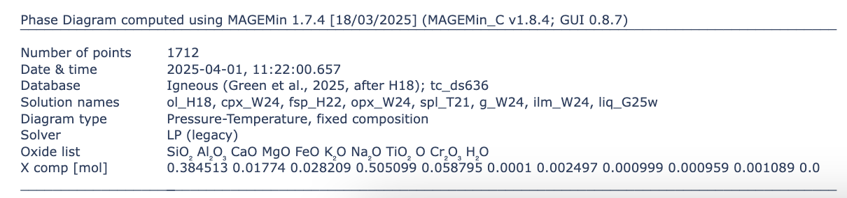
The caption lists useful information such as the version of MAGEMin backend, MAGEMin_C and MAGEMinApp, the activity-composition models, the version of the thermodynamic dataset, the bulk-rock composition and the type of diagram.
Note
The caption is saved together with the figure (as a svg file) when clicking on the little camera icon when hovering your mouse on the top-right corner of the figure.
Note
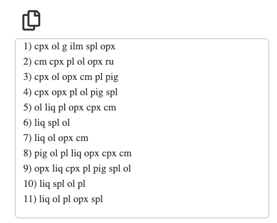
The list of mineral assemblage that cannot be directly labeled on the figure is provided in a text area on the right side of the diagram. The list can be copied by clicking on the Copy button at the top of the list.
Grid point information
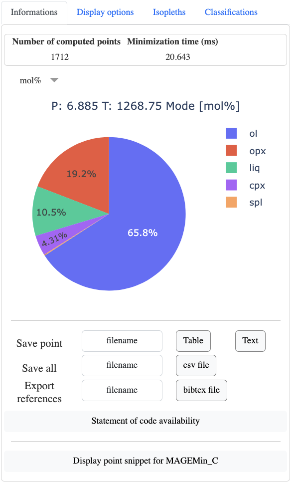
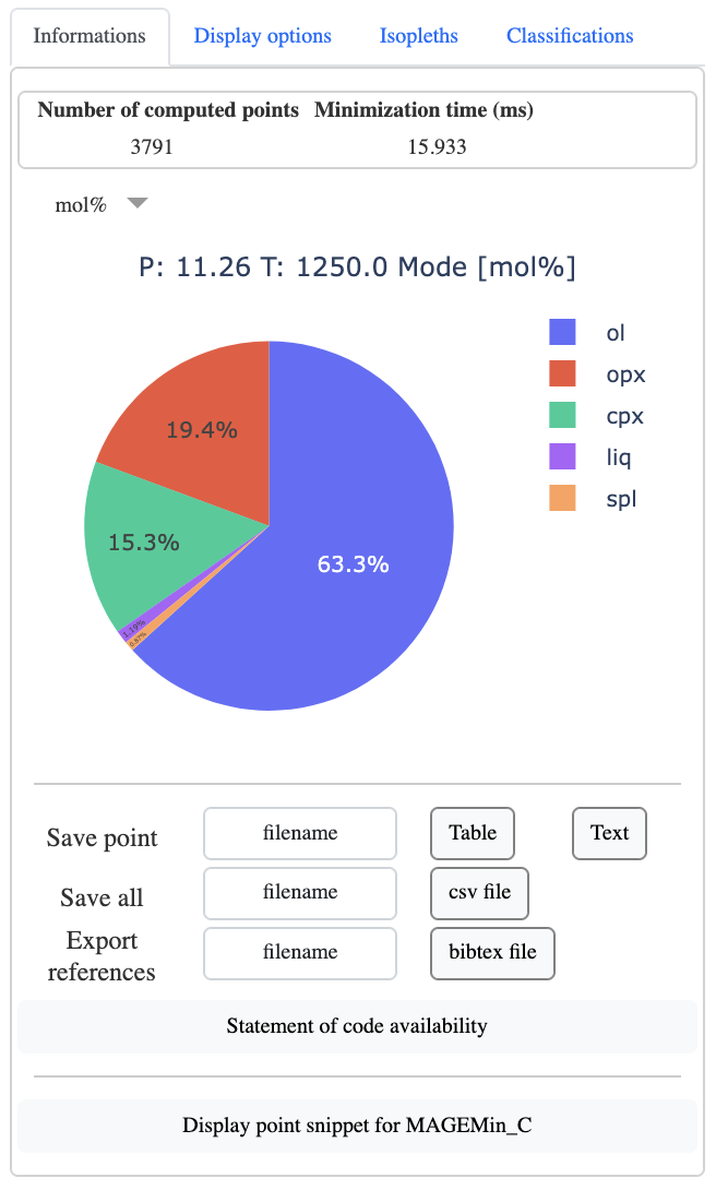
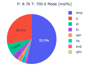
Stable phase mineral fractions and composition can be accessed for any point of the grid by simply clicking on the figure. Doing so will load a pie chart on the right panel in the informations tab:
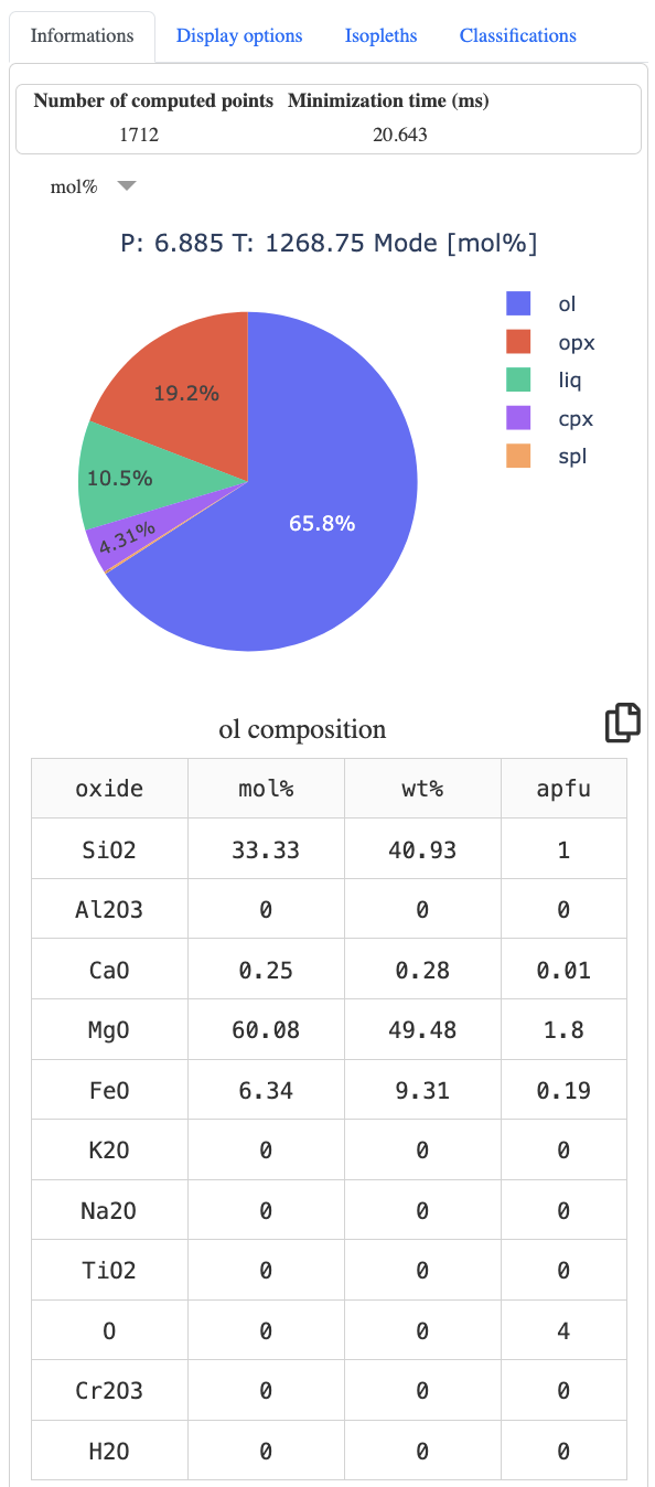
clicking on a mineral of the pie chart will display it's composition:
Refine diagram
In the top-right corner of the figure, there is two buttons allowing you to refine the phase diagram (increase its resolution) using adaptive mesh refinement.
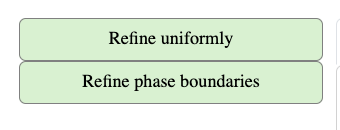
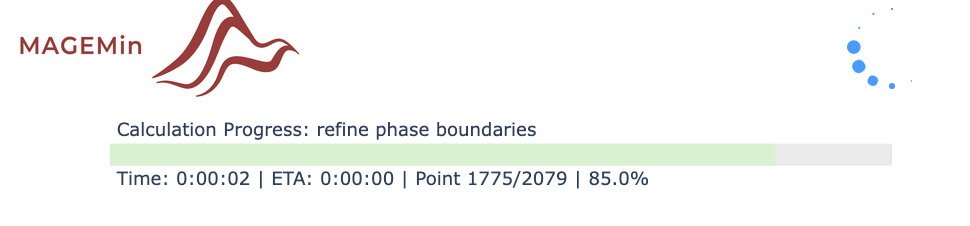
Click on Refine phase boundaries and observe the top-right corner of the App where the progress bar is indicating the number of new points to be computed and the remaining time to completion.
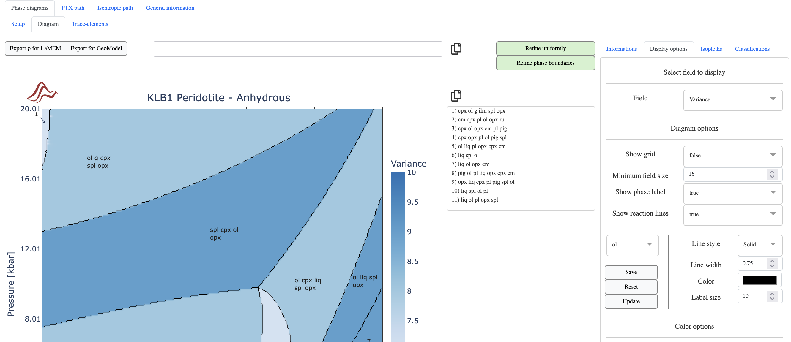
After 2 refinements the updated diagram should look much finer:
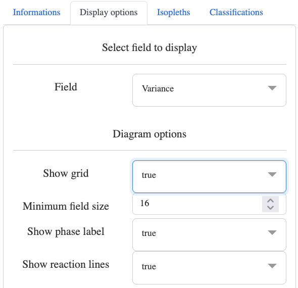
On the right panel, selecting Display options can allow you display the adaptive refinement grid by setting Show grid to true:
which results in:
Note
The size of the cells is decreasing as you get near a reaction line. Here, we use phase boundary as the condition for adaptive mesh refinement but other conditions can be used e.g., dominant endmember fraction.
Uniform refinement adds new points uniformily and not only near reaction lines.
Exporting data
There is two main phase equilibrium data that can be exported: point wise (when clicking on a grid point of the phase diagram) and all points (the full phase diagram).
To export single point data, first click on any point of the grid, then modify the name the file and click on the Table or Text button right next to Save point. For saving all point information, simply provide a filename next to Save all and click on csv file.
Note
Tablesaves the whole output of the stable phase equilibrium whileTextsaves general information.Single point data are downloaded through the web-browser and are likely to end up in your
Downloadsdirectory.Save all points data will end up in the directory indicated in the
Setuptab andGeneral parameterspanel.Mind that when saving all points, the size of file can quickly becomes large (> Go) if the total number of the phase diagram is also large!
2. Reaction lines and isopleths
Reaction lines
Using the previously computed KLB-1 phase diagram, let's now change the liq in reaction line and add isocontours for melt fraction. First make sure you are in the Diagram sub-tab and that you have the Display options panel selected (on the right).
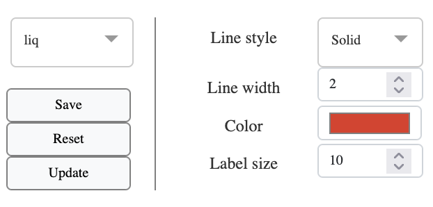
In the Diagram options of the Display options panel, change the selected phase from ol to liq, then change the line width to 2.0 and the color to red. To display the reaction line, simply click on Save then Update:
which should update the phase diagram as follow:

Isopleths
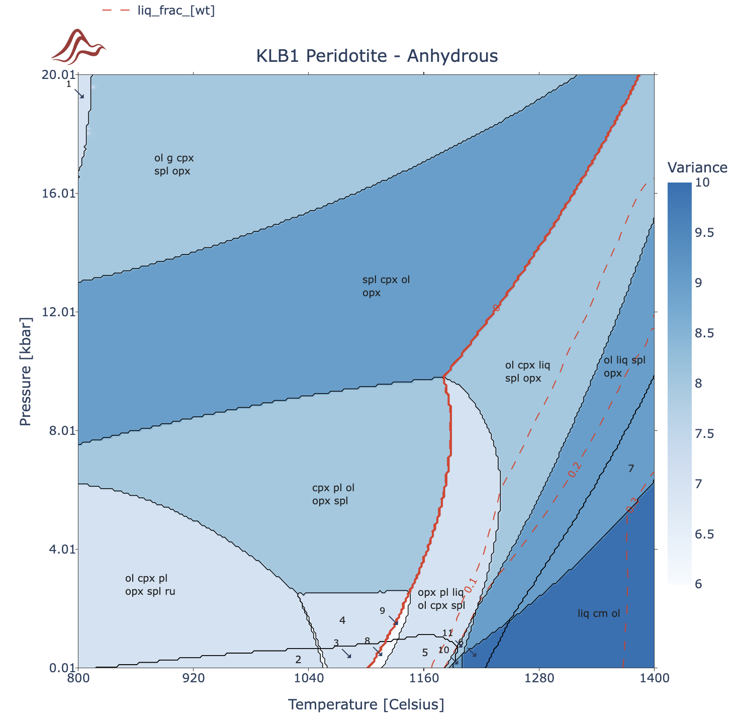
To add isopleths (isocontour), first change the selected right panel from Display options to Isopleths, then choose Isopleth type = solution phase, Phase = liq, Field = mode and Unit = wt. Use the default Rangevalues and set Line style = dash and color to red. Finally click on the Add button:
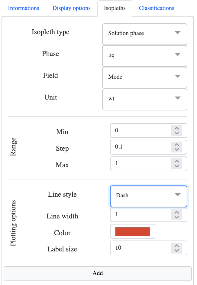
which gives:
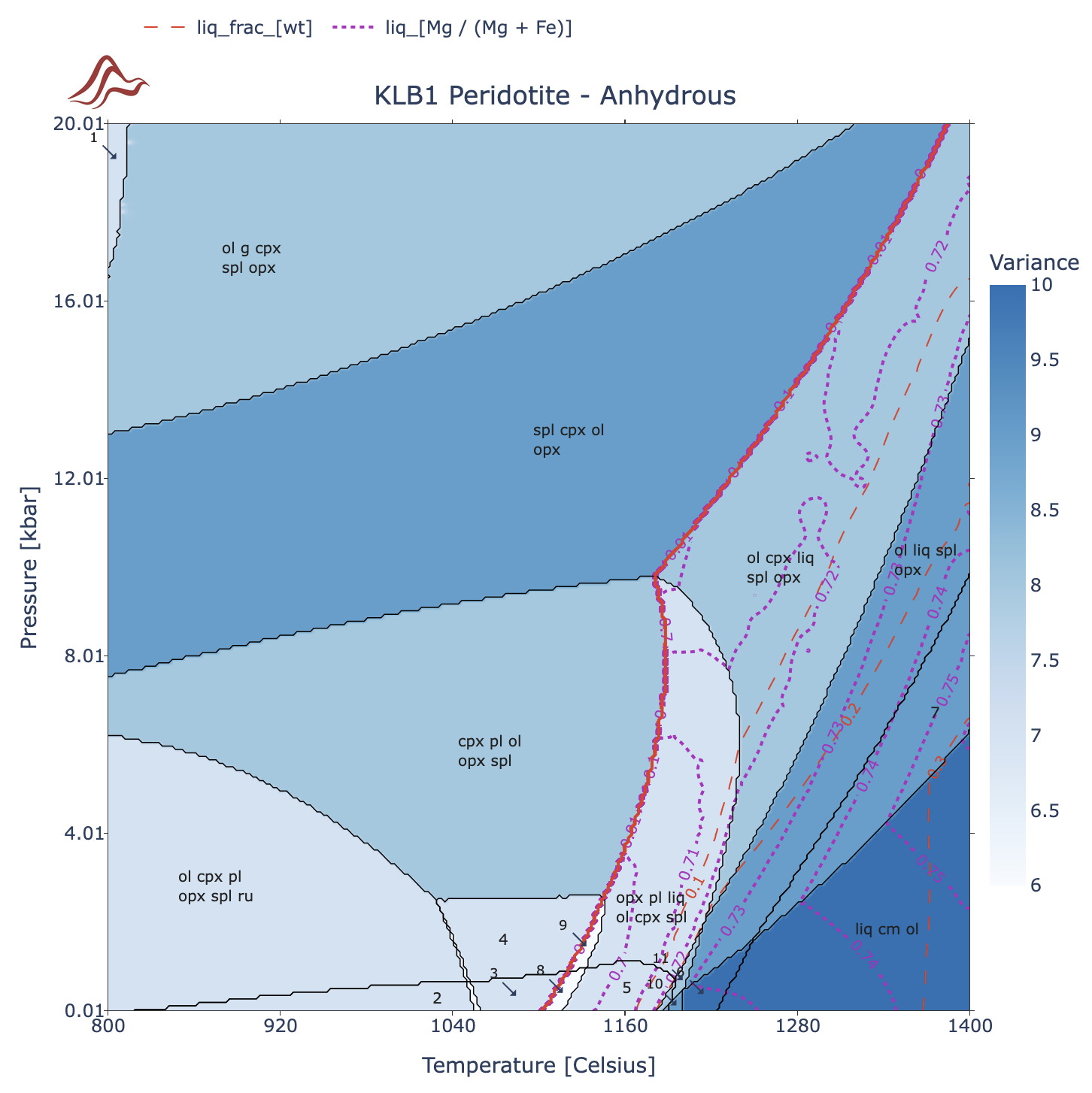
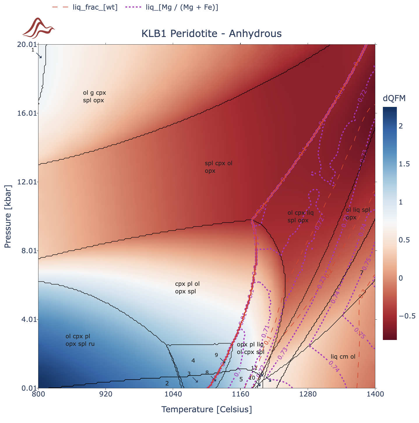
Let's now add isocontour for the Mg# of the liq. Change Field = mode to Field = Calculator apfu which allow you to generate custom atom per formule unit isocontours. In the newly displayed option Calculator (apfu) keep the default value Mg / (Mg + Fe). Then change the Range Stepto 0.01 and the line style and color to your liking:
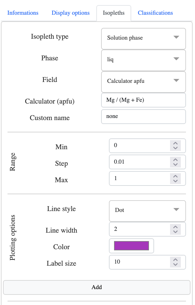
which gives:
Note
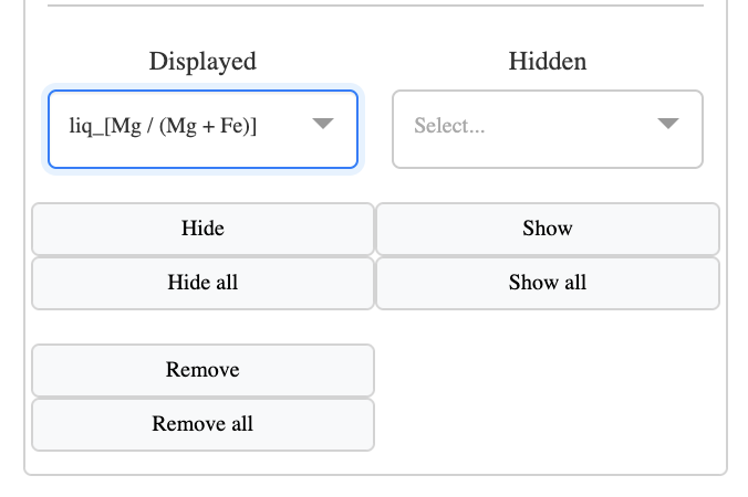
You can manage the isopleths, such as showing/hidding/deleting them in the bottom section of the Isopleths panel:
3. Displayed field and colormap options
You can change the field displayed on the phase diagram by selecting the Display options panel and, for instance, change Field = Variance to Field = log10(dQFM) which will display the Bluescolormap such as for variance. This can be changed in the Color options section located at the bottom of the Display options panel:

For instance, change Colormap = Blues to Colormap = RdBu and the Colormap range from 1-7 to 1-9:

which results in
4. Export figures
Pseudosections, including isopleths and reaction lines can be exported to svg by clicking on the little Camera at the top-right of the diagram:
However, this option merges all the layers together making it difficult to post-process the figures efficiently in any graphic vector software such as Inkscape or Illustrator.
A alternative way to export all layers individually is to use the Export all layers option:
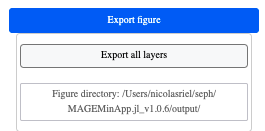
Using the Export all layers option will generate a list of svg files in the output directory of MAGEMinApp:
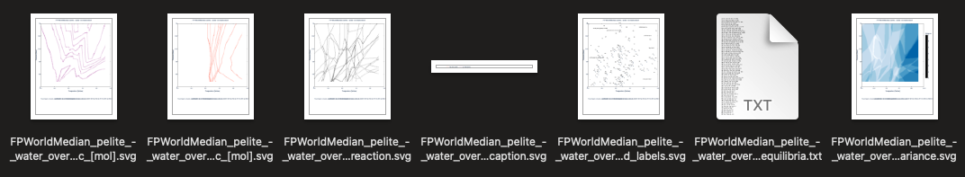
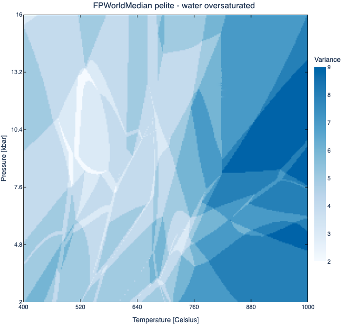
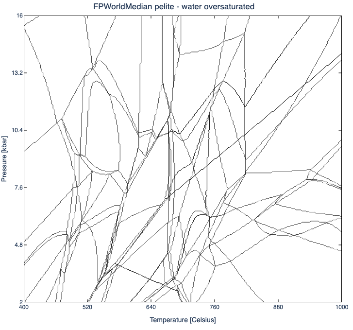
This includes the displayed field (heatmap), the reactions lines, the labels of the phase equilibria (vector and text), a vector file per iso-contour and the iso-contour legends.
Which gives for instance:
5. Deactivate solution and pure phases
In some cases, it is useful to deactivate a solution model (activity-composition model) or a pure phase.
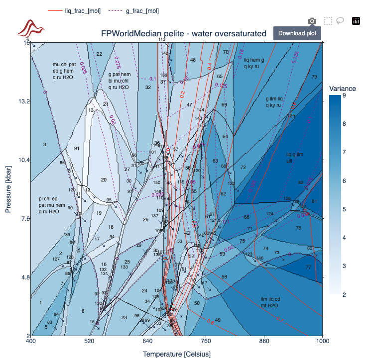
Let's first select the thermodynamic database to be Metapelite (White et al., 2014) and use the default bulk-rock composition FPWorldMedian pelite - water oversaturated. Keep the default diagram type P-T Diagram and pressure range and update the temperature range from 400 to 1000 °C. in the top-left Phase diagram parameters panel, simply click on the rounded button of the Phase selection option, to display the list of available phases for the selection thermodynamic database:

Once the Phase selection panels are unfolded you can provide your custom selection of phases. For instance let's unselect liq, mt and ilmm, and then perform the calculation. Refining the phase diagram twice gives:
Note
- Here, the solution models
liq,mtandilmmare deactivated. However, you can see the phasemtappearing for instance in the large LP-HT (cd+pl+afs+ilm+mt+q+H2O) field. This is because thespmodel can also producemtcompositions.
Warning
When all
Solution phaseare selected, the default combination of phases for the activity-composition set will be applied. In the case of theMetapelitethermodynamic database the default combination fir spinel and ilmenite isspandilm.As soon as one solution model is unselected the default combination is deactivated. This implies that you manually have to select which combination of phase you want and make sure you are not using 2 spinel or 2 ilmenite models at the same time!
6. Buffers
Several buffers can be used to fix the oxygen fugacity
qfm-> quartz-fayalite-magnetiteqif-> quartz-iron-fayalitenno-> nickel-nickel oxidehm-> hematite-magnetiteiw-> iron-wüstitecco-> carbon dioxide-carbon
Similarly activity can be fixed for the following oxides
aH2O-> using water as reference phaseaO2-> using dioxygen as reference phaseaMgO-> using periclase as reference phaseaFeO-> using ferropericlase as reference phaseaAl2O3-> using corundum as reference phaseaTiO2-> using rutile as reference phaseaSiO2-> using quartz/coesite as reference phase
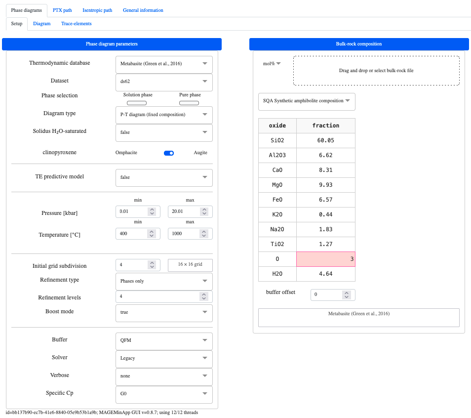
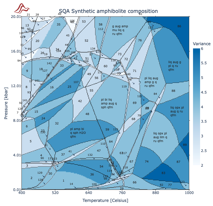
Let's compute a P-T diagram using the qfm buffer. For instance, select the thermodynamic database to be Metabasite (Green et al., 2016). Choose the pressure-temperature range of your choice. Select SQA synthethic amphibolitic composition in the middle Bulk-rock composition panel, then in the Phase diagram parameters left panel, select Buffer = QFM. Finally, make sure you saturate the bulk-rock in O by changing the value to 3.0:
Which gives, after 4 levels of refinements:
Note
If you click on any point of the diagram, you can see in the
Informationspanel, that every field contain aqfmphase. This phase has a fraction equal to 0.0 and simply shows that the system is buffered.If one of the field does not have the buffer phase, it indicates that not enough free
Ohas been provided.
Warning
- The
Buffer offsetoption in theBulk-rock compositionpanel is used to offset the oxygen buffer in thescale, while for activity it serves as the activity value.
7. Latent heat of reaction
Heat capacity is computed as a second order derivative of the Gibbs energy with respect to temperature using numerical differentiation.
There is however two ways to retrieve the second order derivative: 2. Default option Specific Cp = G0 - no latent heat of reaction: Fixing the phase assemblage (phase proportions and compositions) and computing the Gibbs energy of the assemblage at T, T+eps and T-eps.
- Full differentiation option
Specific Cp = G_system- latent heat of reaction: Computing three stable phase equilibrium at T, T+eps and T-eps.
Note
- While the first method is computationally more efficient, it does not account for the latent heat of reaction. When having correct heat budget is important it is therefore recommanded to employ the second approach.
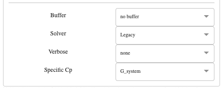
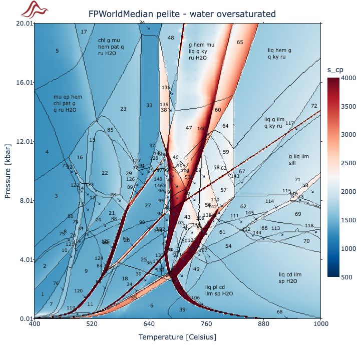
To compute a phase diagram that takes into account latent heat reaction simply choose Specific Cp = G_system in the Phase diagram parameters panel:
Using the metapelite database and the FPWorldMedian pelite - oversaturated composition and 4 levels of refinement, together with displaying s_cp (and capping max value to 4000 for the colormap) gives:
Note
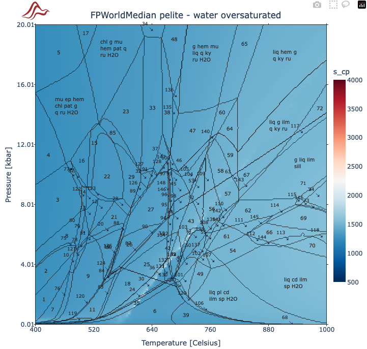
- Without accounting for latent heat of reaction (
Specific Cp = G0), the values of the specific heat capacity are drastically different:
8. Trace element modelling
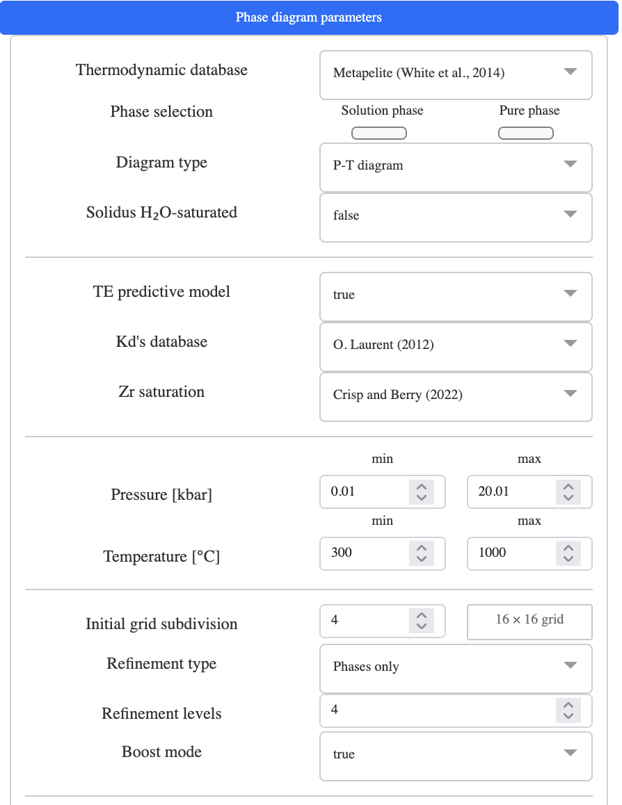
Let's predict trace-element partitioning together with a new phase diagram using the metapelite database (White et al., 2014) and the pre-defined World Median Pelite oversaturated.
Details
Thermodynamic database -> Metapelite
Diagram type -> P-T diagram
TE predictive model -> true
Pressure -> 0.01 to 10.0 kbar
Temperature -> 300.0 to 1000.0 °C
Initial grid subdivision -> 4
Refinement levels -> 4
Trace-element composition panel -> select default
tonalite
Which after performing the calculation should result in:
Now move to the Trace-elements sub-tab, and to load the trace-element prediction, click on the button Load/Reload trace-elements. Doing so will display the default field Sat_zr_liq, which is the computation saturation level of liquid for zirconium in ug/g. To change the displayed field navigate to the Display options panel on the right side and choose Field type = Trace element ansd click Compute and display.
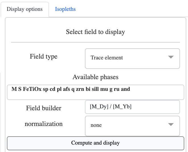
which will display (using default options) the ratio
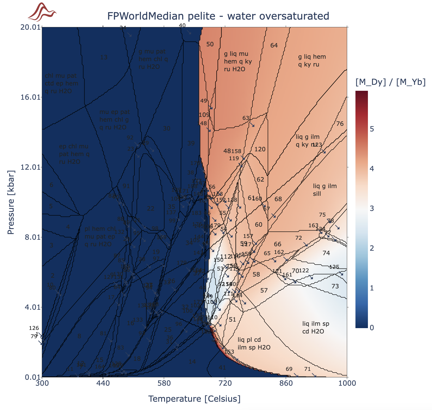
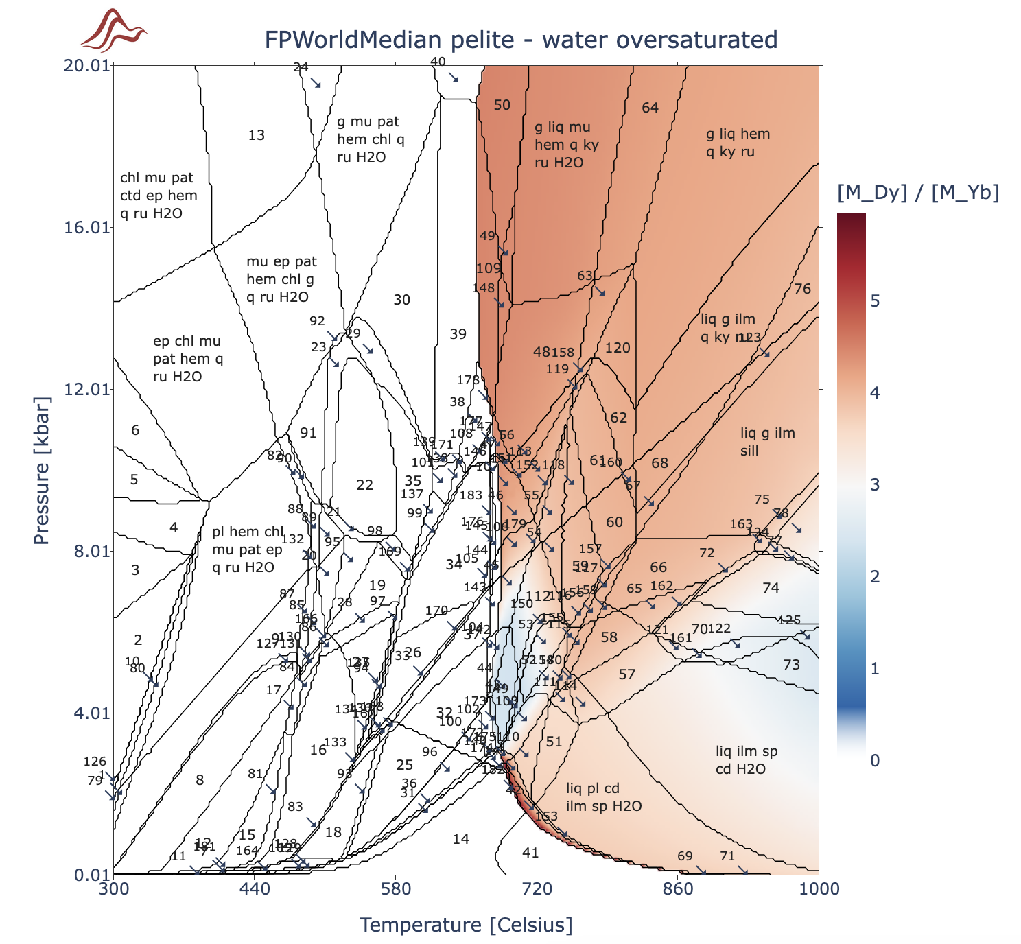
To make the melt-free transparent in colormap, you can change in the Color options section of the Display options panel Set min to white = true which yields:
Display trace-element spectrum
In order to display trace-element spectrum from any suprasolids point of the computed grid, simply click on the grid. Doing so will display a spectrum in the figure right above the trace-element diagram:
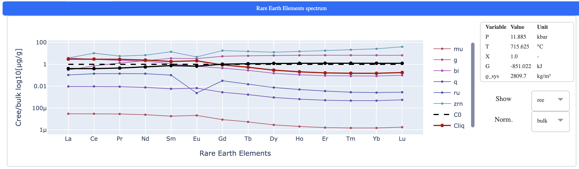
Tip
In the trace-element spectrum panel, you can change the display elements from
reetoalland change the normalization method frombulktochondrite.As for other
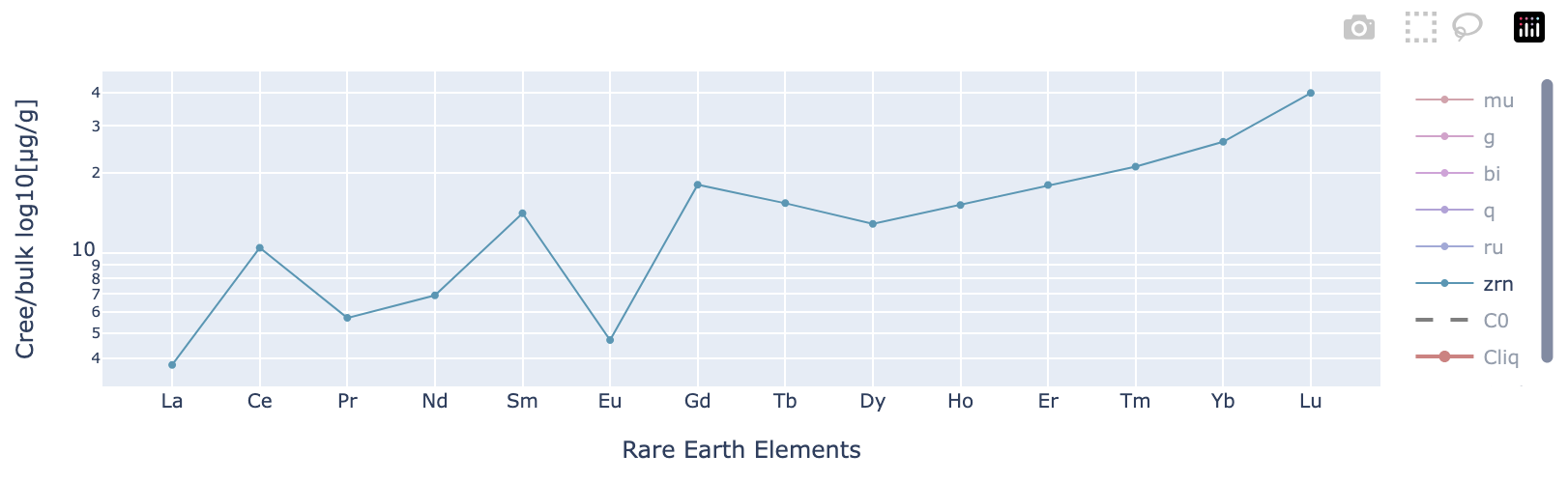
MAGEMinAppfigures, you can export the spectrum by hovering your cursor in the top-right corner of the figure and clikc on the small camera icon. This will save an*.svgvector graphic file.Double-clicking on a phase abbreviation on the right legend of the spectrum will isolated the selected spectrum:
9. Solidus H2O saturated phase diagram
To compute solidus H₂O-saturated phase diagram, let's (for instance) change the thermodynamic database to Metabasite (Green et al., 2016), choose Solidus H₂O-saturated = true, select clinopyroxene = aug:
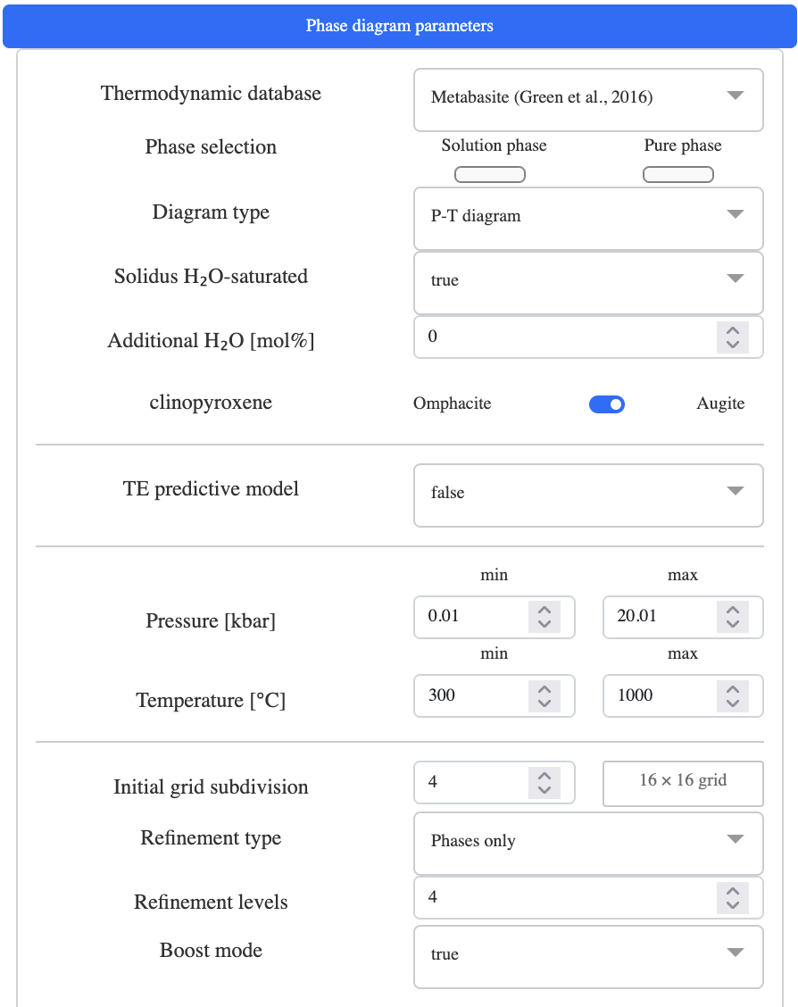
in the middle Bulk-rock conmposition panel, select SM89 oxidised average MORB composition and change the water-content from 20.0 to 40.0 to ensure water-saturation

Computing the diagram and displaying the system H₂O-activity should gives:
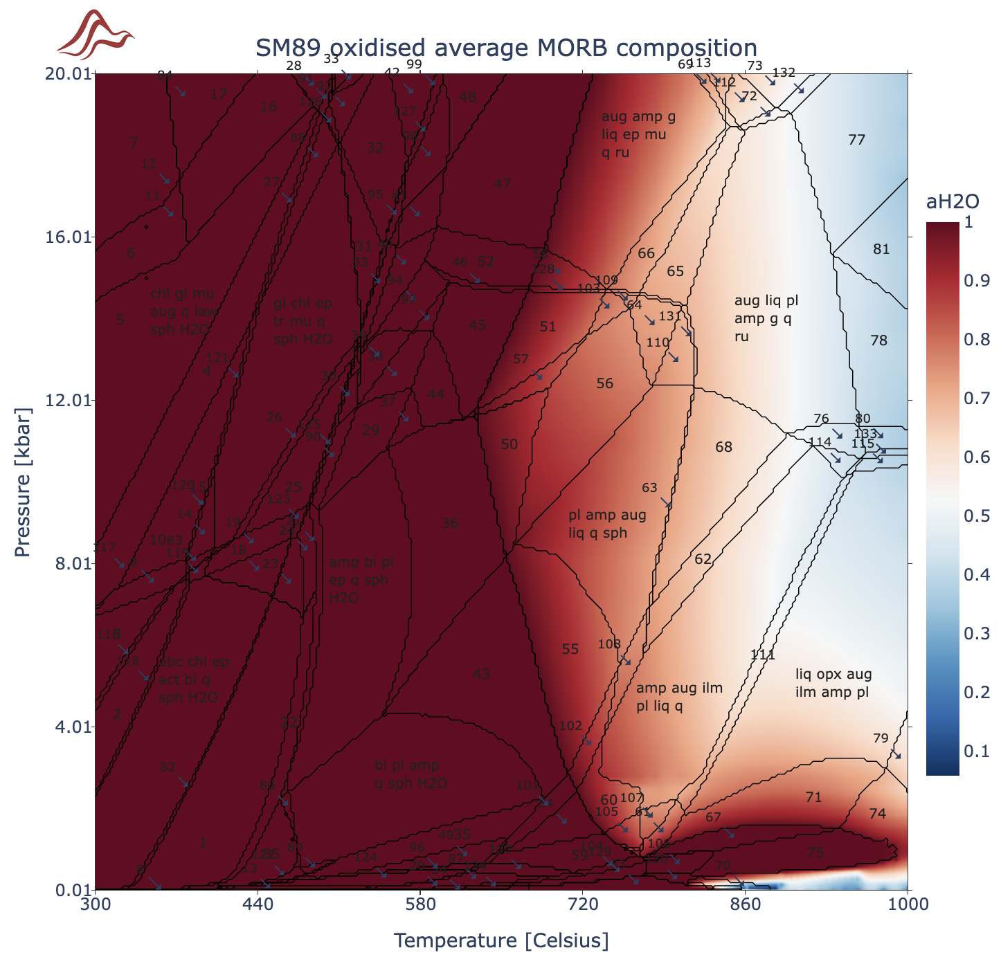
Note
First, for the given pressure range (and using 50 pressure steps), the water-saturated solidus is extracted using bisection method. Subsequently, the pressure-dependent solidus temperature is interpolated using PChip interpolant. At Tsuprasolidus = Tsolidus + 0.01 K, a second interpolation is used to retrieve the amount of water saturating the melt. The latter interpolant is then used to prescribe the water content of the bulk, ensuring pressure-dependent water saturation at solidus (+ 0.1 K).
Extra water can be added in the
Phase diagram parameterpanel, using the optionAdditional H₂O [mol%].
10. TX fixed pressure diagram
The objective of T-X diagram is to fix the pressure while having in the vertical axis a range of temperature and on the horizontal axis a varying bulk-rock composition. Variation in the bulk-rock composition can be applied to any oxides and the two end-member bulk-rock composition added to bulk-rock input file (see Bulk-rock input file).
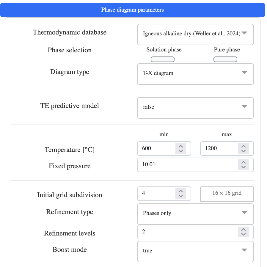
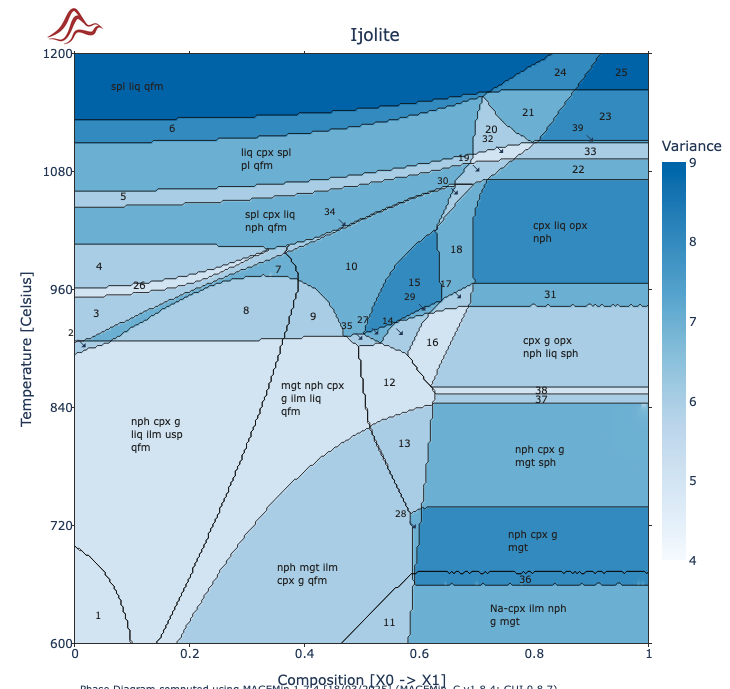
To compute a T-X with fixed pressure diagram, simply select in the Setup sub-tab Diagram = T-X diagram. For instance, choose the Igneous alkaline dry thermodynamic database (Weller et al., 2024) and change the temperature range to 600 - 1200 °C. Keep the default fixed pressure at 10.0 kbar:
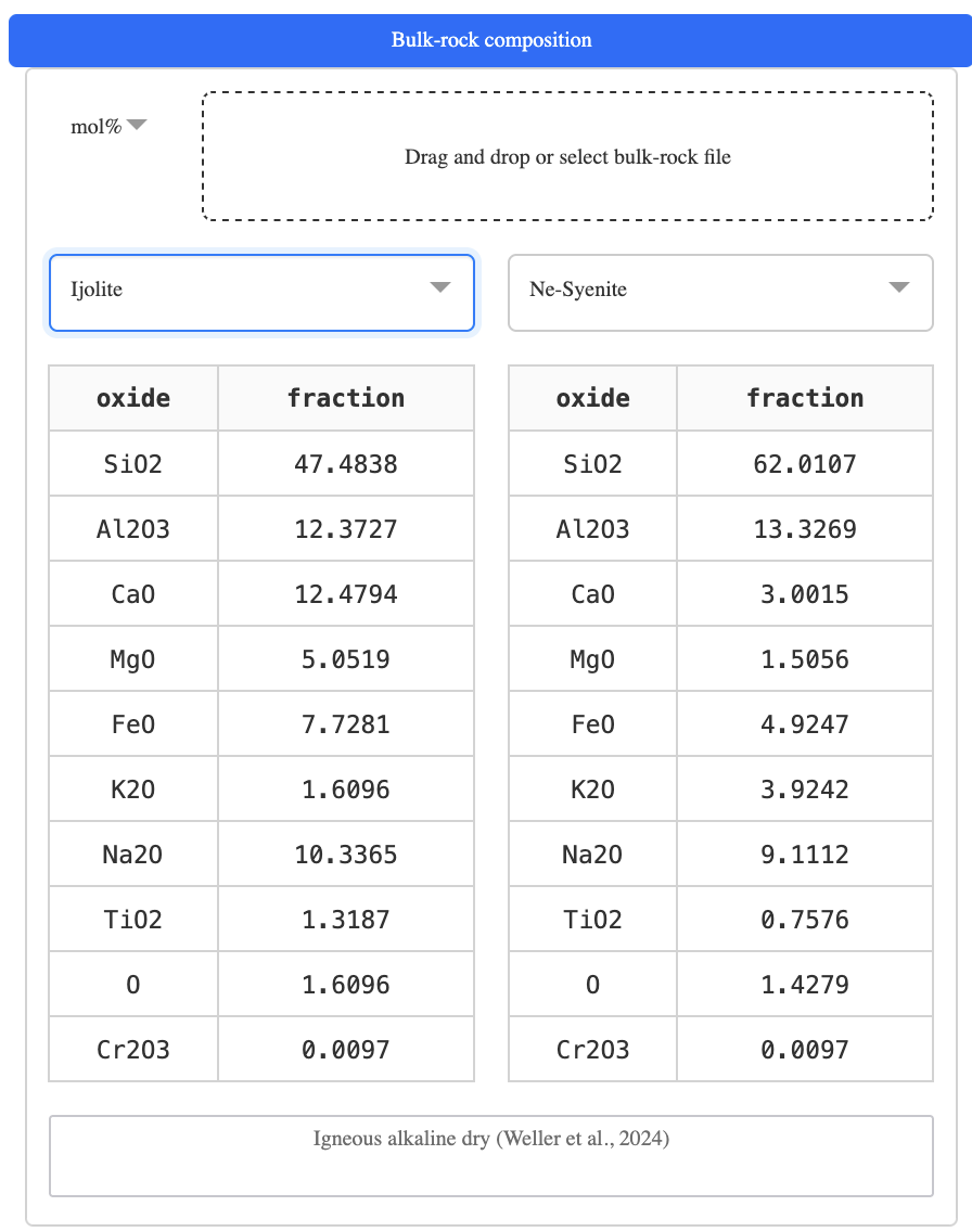
In the middle Bulk-rock composition panel select the predefined Ijolite bulk composition for the left table, and the Ne-Syenite bulk composition for the right table.
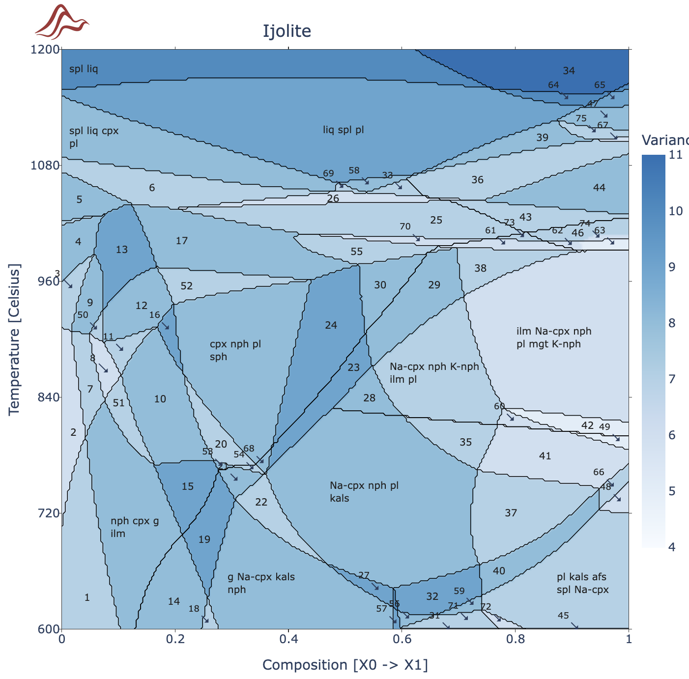
Compute the diagram with Initial grid subdivision = 5 and Refinement levels = 3:

Note
Some of the reaction lines in the high temperature part of the diagram are not perfectly clean. This problem is related to the use of the
Boost modewhich uses the results of the previous refinement level as an initial guess for the next level.In this case, performing the calculation with
Boost mode = falsefixed the problem:
Tip
- In some cases, when
Boost mode = true, the produced diagram will display some poorly resolved reaction lines. To fix this you can either increase the initial grid subdivisionInitial grid subdivision = 5or setBoost mode = false.
T-X buffer
Previously we changed the composition from Ijolite to Ne-Syenite. Let's instead vary the qfm buffer offset for Ijolite composition from -5 to 5.
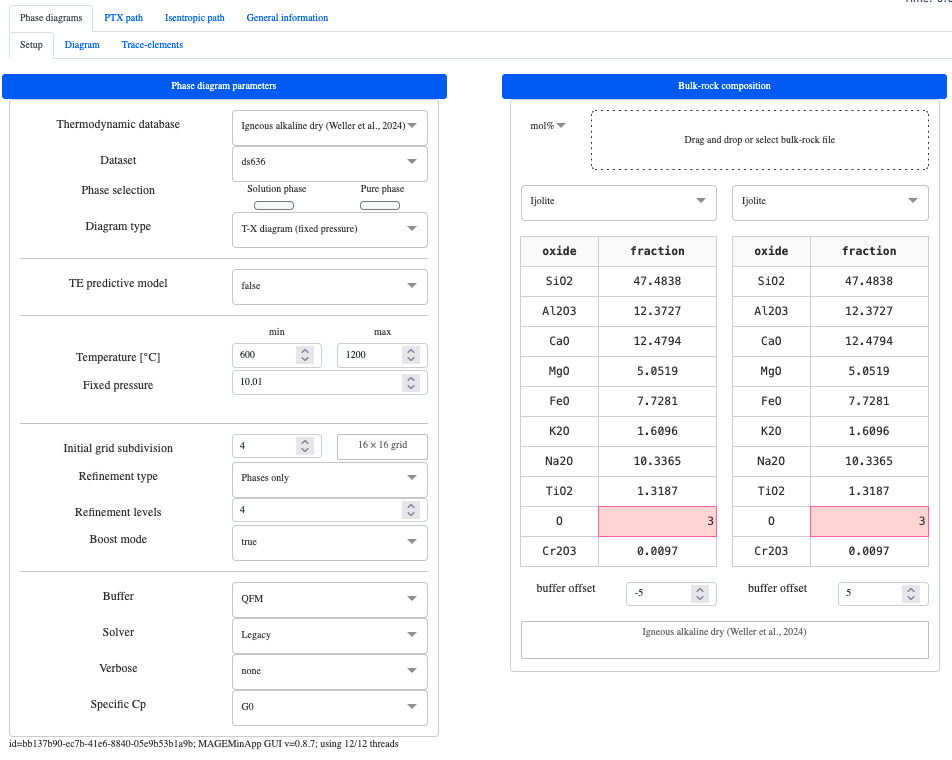
In the Phase diagram parameters left panel, select Buffer = QFM, then in the middle Bulk-rock composition panel, select Ijolite for both left and right composition. Then change Buffer offset to -5 for the left entry, and to 5 for the right entry. Don't forget to increase the O content, for isntance to 3.0:
Which after 4 levels of refinements results in:
Warning
- Here, you can see that we did not provide enough
Oasqfmphase does not appear on the right side of the diagram. You can easely fix that by change theOvalue to 10 and relaunch the calculation
Fixing the O content and contouring

11. PTX diagram
PT-X diagrams differ from P-X and T-X diagrams in the sense that both pressure and temperature can be varied along a pressure-temperature path. This option can be particularily useful when modelling subduction geotherm for instance.
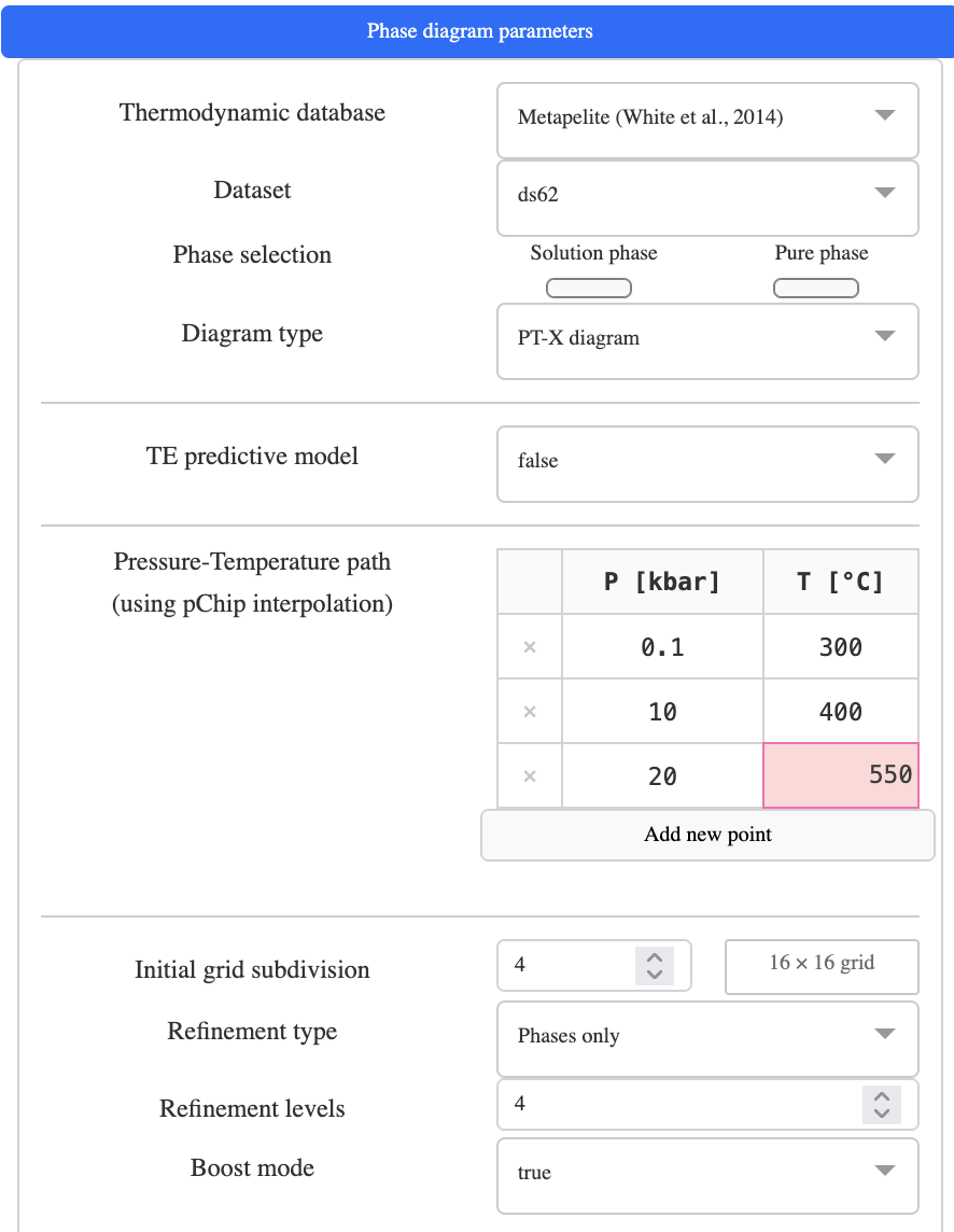
To perform a PT-X diagram, let's first select the Metapelite database (White et al., 2014) and set Diagram type = PT-X diagram. When PT-X diagram is selected, a new panel with a list of pressure-temperature points becomes available. Let us define a few point as to roughly simulate a subduction pressure-temperature path:
| Pressure | Temperature |
|---|---|
| 0.1 | 300.0 |
| 10.0 | 400.0 |
| 20.0 | 550.0 |
Your Phase diagram parameter left panel should look like:
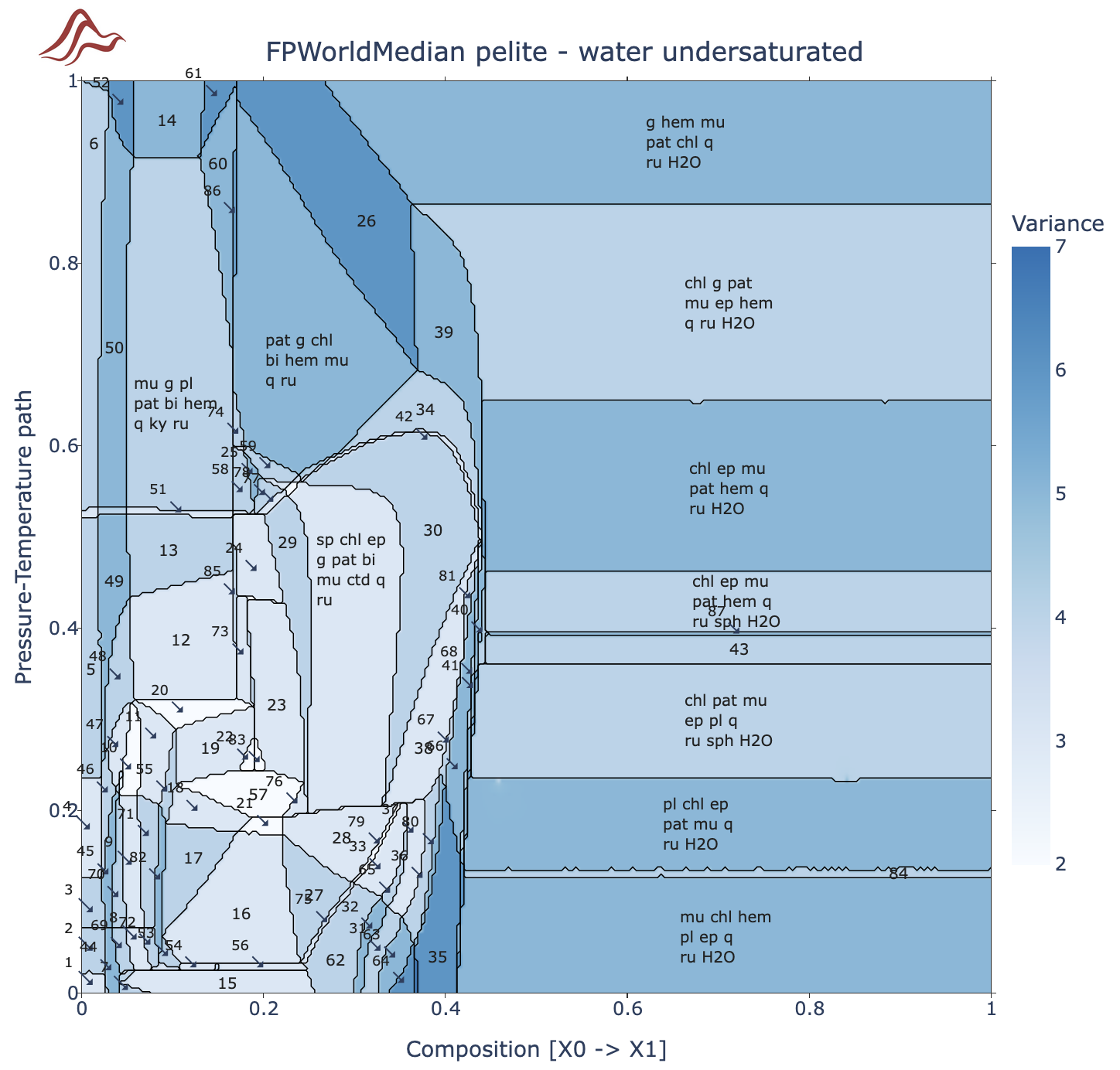
Then in the Bulk-rock composition middle panel, select the pre-defined bulk FPWorldMedian pelite undersaturated for the left table and FPWorldMedian pelite oversaturated for the right table. Select Refinement levels = 4 then compute the diagram:
12. TT polymetamorphic diagram
The goal of a T-T poly-metamorphic diagram is to predict the evolution of the stable phase assemblage for a rock undergoing two successive metamorphic events.
During the first metamorphic event, the starting bulk-rock composition is used to compute the first stable phase equilibrium at the minimum temperature (and given fixed pressure). In the event free water is predicted, it is removed from the bulk, so that the system become water-saturated. This is repeated for every temperature step until reaching the provided maximum temperature. In a similar manner, when crossing the solidus, melt can be removed according to two options:
Liq extract threshold [vol%]which is the threshold invol%over whichliqwill extracted.Remaining liq fraction [vol%]which the volume ofliqleft after extraction.
Note
Liq extract threshold [vol%]andRemaining liq fraction [vol%]can both be set for metamorphic event 1 and 2.Make sure your starting bulk-rock composition is water oversaturated.
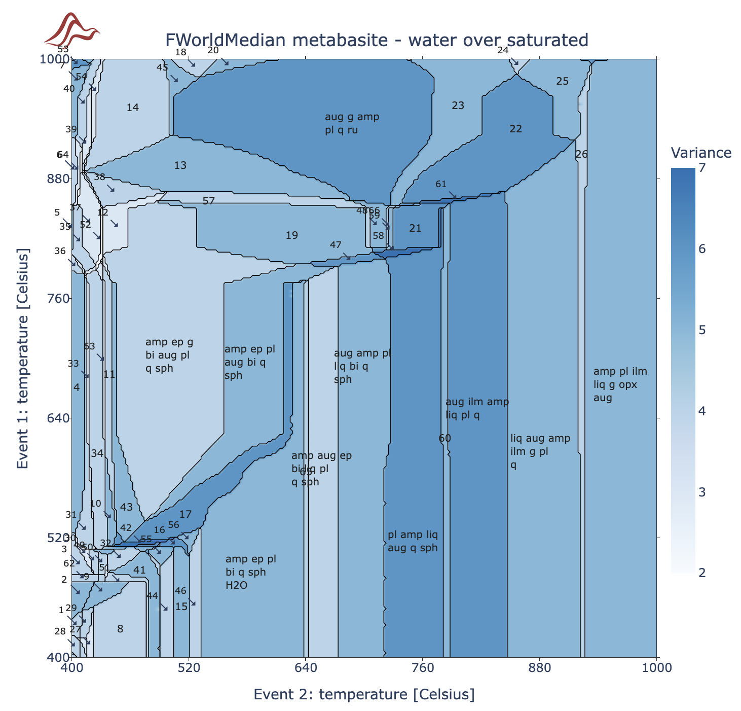
Let's try it out! First, select the Metabasite database (Green et al., 2016) and the FWorldMedian metabasite oversaturated pre-defined composition. Then Diagram type = T-T (poly-metamorphic), and clinopyroxene = Augite. You can keep the default values for the fixed pressure (10.0 kbar) and the temperature range of metamorphic events 1 and 2 (400 - 1000 and 400 - 1000 °C):
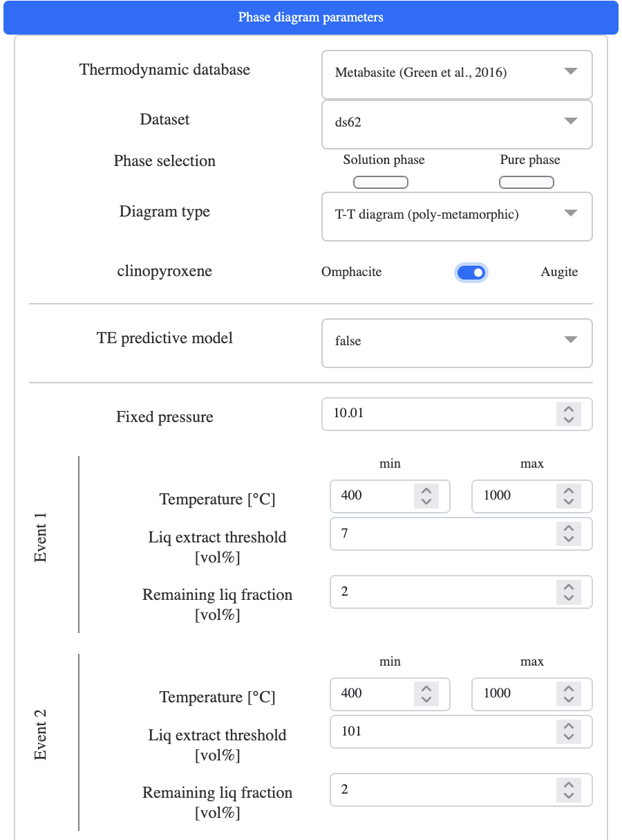
For the first event, you can see that the Liq extract threshold [vol%] is set to 7.0 while Remaining liq fraction [vol%] is set to 2.0. For the second event Liq extract threshold [vol%] is set to 101, which simply deactivate liq extraction.
Compute the diagram which should give:
Note
- At very high temperature extracting nearly all the melt may become a problem as you are left with highly refractory compositions. In this case you either leave slightly more melt in the host-rock or decrease the maximum temperature.
13. LaMEM density diagram
Quickstart
When computing a density diagram for LaMEM geodynamic modelling code, the initial grid setup needs to be changed. Density diagrams for geodynamic modelling generally need to evenly sample the pressure-temperature space of interest and should avoid using refinement. The recommanded mesh configuration in the Setup panel is the following.
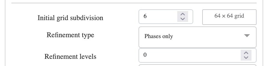
which when displaying the grid and the system density gives:

To export the diagram in the format used in LaMEM (*.in), simply click on the top-left Export rho for LaMEM button!
Note
Ensure that the thermodynamic you select is calibrated for your pressure-temperature of interest.
Make sure the diagram you produce cover the pressure-temperature you expect in your geodynamic simulation. Otherwise
LaMEMwill extrapolate to out of bound regions which may not be what you want!With the above configuration, the total number of computed points will be 4225 which is largely sufficient. Mind that
LaMEMdoes not support density diagram with a number of points greater than ~20k.
Upper mantle density diagram
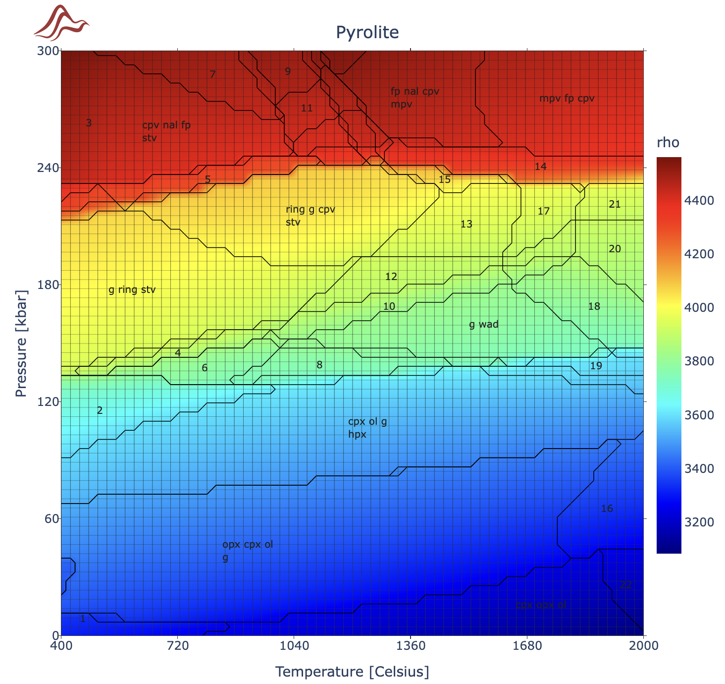
When modeling plate-tectonics dynamics, one generally wants to account for phase change in the mantle. To produce a density diagram for the upper mantle you can use the Mantle database (Holland et al., 2012) or mtl acronym and the pre-defined pyrolite composition. A possible set of pressure-temperature valid for the lithosphere and the asthenosphere is for instance, from 1 to 300 kbar (0.1 to 30 GPa) and from 400 to 2000 °C.
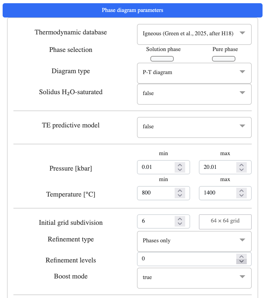
This results in the following upper mantle density diagram that can be exported for LaMEM
14. Draw a P-T path on the diagram
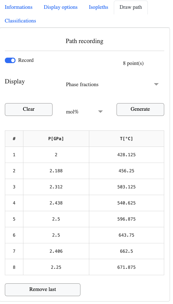
The Draw path panel (available in the Diagram sub-tab, right sidebar) lets you manually trace a P-T path directly on the phase diagram by clicking on grid points, and then generates a stacked area chart of phase fractions along that path.
Step 1 - Enable recording
Open the Draw path panel on the right sidebar. Toggle Record to on. The point counter resets to 0 point(s).
Note
Recording is automatically disabled when you switch away from the Draw path panel.
Step 2 - Click points on the diagram
With Record active, click on any location of the phase diagram. Each click appends a new row to the path table showing the coordinates of the selected point:
| # | P [kbar] | T [°C] |
|---|---|---|
| 1 | … | … |
| 2 | … | … |
| … | … | … |
Use
Remove lastto delete the most recently added point.Use
Clearto discard the entire path and start over.
Note
For P-X and T-X diagram types the table columns adapt accordingly (X; P [kbar] or X; T [°C]).
Step 3 - Choose the output unit and generate
Select the system unit for the phase fractions plot:
| Unit | Description |
|---|---|
mol% | Molar fractions |
wt% | Weight fractions |
vol% | Volume fractions |
Click Generate. MAGEMinApp computes the stable phase equilibrium at each recorded point and displays a stacked area chart titled Phase fractions along path in the expandable canvas below the controls.
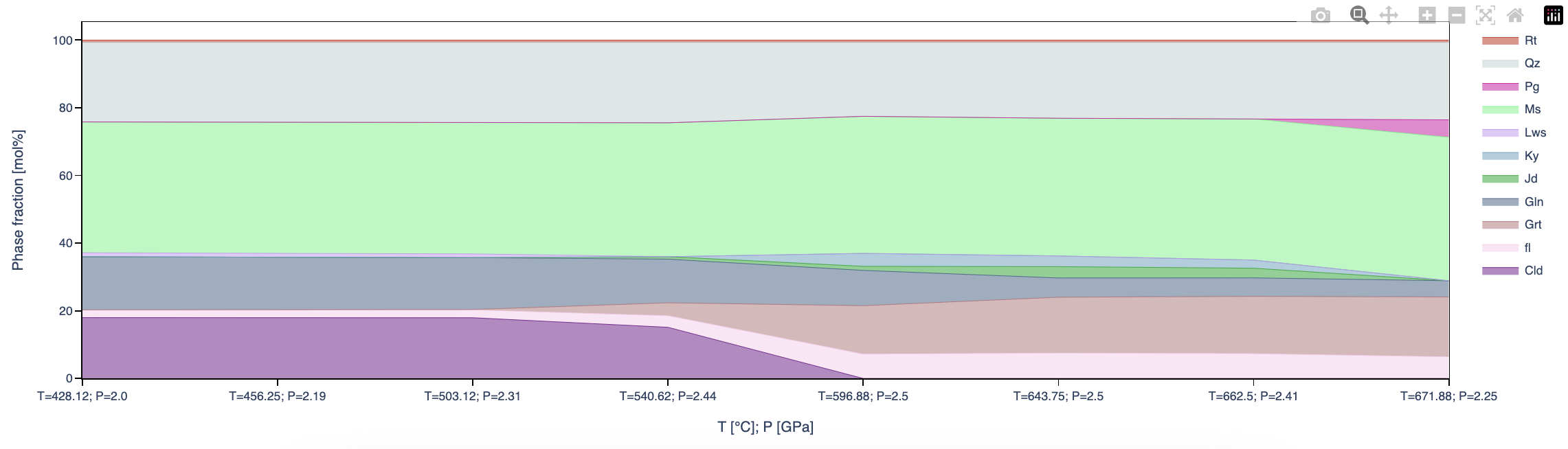
The x-axis reports the path coordinates (T [°C]; P [kbar] for a P-T diagram) and the y-axis shows the phase fraction in the selected unit. The chart can be exported as an svg file using the camera icon in the top-right corner of the plot.
15. Quantitative isopleth thermobarometry with IntersecT
The IntersecT tab implements quantitative isopleth thermobarometry (Nerone et al., 2025, doi:10.1016/j.cageo.2025.105949), following the compositional-quality-factor (Q
This tutorial reuses the two example files shipped in examples/IntersecT/ of MAGEMinApp:
Petroccia_et_al_2025_bulk_Magemin.csv- a bulk-rock input file (same format as described in Bulk-rock input file) containing one custom composition namedBAR38A.BAR38A_measurements_julia.csv- a measured mineral-composition file for the same sample, with one row of observed a.p.f.u. values and one row of analytical uncertainties for garnet (Grt), chloritoid (Cld) and muscovite (Ms).
Step 1 - Load the bulk-rock composition and compute a phase diagram
BAR38A is a peraluminous, water-bearing pelite intended for the Metapelite extended (White et al., 2014; Green et al., 2016; Evans & Frost, 2021) thermodynamic database, acronym mpe.
Warning
Before doing anything else, open the Setup tab, General parameters panel, and set Mineral names = Warr (2021). IntersecT matches phases between the measurement file (column headers such as Grt_Mg) and the computed grid using the IMA-CNMNC symbols of Warr (2021). With the default Legacy naming (MAGEMin's internal codes, e.g. g, ctd, mu) no phase will be found in common and the Stable phases checklist will stay empty.
In the Phase diagram tab, Setup sub-tab: 2. In Phase diagram parameters, set Database = Metapelite extended (White et al., 2014, Green et al., 2016, Evans & Frost., 2021).
In
Bulk-rock composition, drag and dropPetroccia_et_al_2025_bulk_Magemin.csvonto the upload field. ABulk-rock(s) composition(s) successfully loadedalert confirms the import.Still in
Bulk-rock composition, selectBAR38Ain the dropdown above the composition table (it is appended at the end of the list for thempedatabase).Since
BAR38Ais a peak-pressure, chloritoid-and-garnet-bearing pelite, lower the default temperature range to something like 400 – 700 °C (the default 800 – 1400 °C window is too hot forCldto be stable). Change pressure range (15 - 35 kbar).Set
Initial grid subdivision = 4andRefinement levels = 3, then clickCompute phase diagram.
Note
If Cld, Grt and Ms do not all appear together anywhere on the resulting diagram, widen or shift the pressure-temperature window and recompute - IntersecT can only be run on phases that are present, in common with the measurement file, somewhere on the grid.
Step 2 - Load the measurement file and select the stable phases
Switch to the top-level IntersecT tab (Setup panel on the left, open by default).
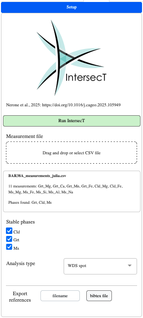
Drag and drop
BAR38A_measurements_julia.csvonto theMeasurement fileupload field.The panel below the upload field reports the file name, the number of measured columns and the phases found in the header (
Grt,Cld,Ms):
| Column | Phase | Element (a.p.f.u.) |
|---|---|---|
Grt_Mg, Grt_Ca, Grt_Mn, Grt_Fe | Garnet | Mg, Ca, Mn, Fe |
Cld_Mg, Cld_Fe | Chloritoid | Mg, Fe |
Ms_Mg, Ms_Fe, Ms_Si, Ms_Al, Ms_Na | Muscovite | Mg, Fe, Si, Al, Na |
The first data row holds the observed a.p.f.u. values, the second row the corresponding analytical uncertainties.
The
Stable phaseschecklist is automatically populated with the phases found both in the measurement file and on the computed grid, and all of them are pre-checked. Uncheck a phase here to exclude it from the calculation.Leave
Analysis type = WDS spot(or pickWDS map/EDS). This setting is only used to auto-estimate the analytical uncertainty when the measurement file does not already provide one - sinceBAR38A_measurements_julia.csvalready has an explicit uncertainty row, it has no effect on this particular run, but the field must still hold a valid value.
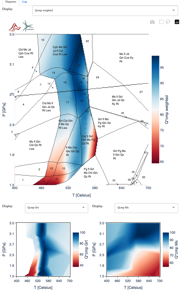
Step 3 - Run IntersecT and compute the Q factor
Click Run IntersecT. For each selected phase, IntersecT compares the modelled a.p.f.u. composition at every grid point to the measured value (weighted by its uncertainty), giving a compositional quality factor Q
The Display dropdown above the main diagram (Diagrams sub-tab) is populated with all available fields and defaults to Qcmp weighted:
| Field | Meaning |
|---|---|
Qcmp weighted / Qcmp unweighted | Combined quality factor over all selected phases (weighted by each phase's best-fit reduced- |
redchi2 total | Combined reduced- |
Qcmp <phase> / redchi2 <phase> | Quality factor / reduced-Qcmp Grt |
Qcmp <Phase_Element> | Quality factor for a single measured a.p.f.u. column, e.g. Qcmp Grt_Mg |
The two smaller diagrams below let you compare two more fields side by side (e.g. Qcmp Grt against Qcmp Cld) to see whether all phases agree on the same pressure-temperature region.
Note
Switching the displayed field automatically rescales Min/Max in the Color options panel to that field's range, since Qcmp and redchi² fields have very different scales.
Step 4 - Read the Log
Open the Log sub-tab to get the full text report: for each selected phase and for each measured element, the (P,T) location and value of the maximum Q
Step 5 - Overlay isocontours (optional)
In the Options column, the Isocontours section works as in the Phase diagram tab (see 2. Reaction lines and isopleths), with two contour sources:
Type = Measurements: contour a modelled a.p.f.u. field for aPhase/Elementpair found in the measurement file, e.g.Phase = Grt,Element = Mg.Type = Field: contour one of theIntersecTresult fields listed in theFielddropdown (only available afterRun IntersecT), e.g.Field = Qcmp weightedwithMin = 0,Step = 0.1,Max = 1to outline, for instance, the Q≥ 0.8 region.
Set Range, line style/width/size and color to your liking and click Add. Added isocontours can be shown, hidden or removed from the Displayed/Hidden lists at the bottom of the panel, exactly as for the regular phase-diagram isopleths.
Tip
Overlaying a Measurements-type isocontour for the same Phase_Element used in the fit (e.g. Grt_Mg) directly on top of the Qcmp field is a quick way to check, visually, which part of the high-Q region is actually controlled by that particular element.