MAGEMin_C.jl: Tutorials

This page provides a set of detailed tutorials showing how to use MAGEMin_C.jl to perform phase equilibrium calculations.

Info

• Iterative phase equilibrium calculation

• Single point trace element partitioning

• Trace element partitioning

Note

• The tutorials are not optimized for performances, but are provided in hope they can be useful to present MAGEMin_C functionality.

Iterative phase equilibrium calculation

first add MAGEMin_C and Plots

julia> ] add MAGEMin_C
julia> ] add Plots

and use MAGEMin_C and Plots as:

using MAGEMin_C, Plots

First let's first initialize MAGEMin with the metapelite database (White et al ., 2014)

data        =   Initialize_MAGEMin("mp", verbose=false);

Then define the bulk-rock composition (wt fraction) the related oxide list and the system unit

X           = [0.5922, 0.1813, 0.006, 0.0223, 0.0633, 0.0365, 0.0127, 0.0084, 0.0016, 0.0007, 0.075]
Xoxides     = ["SiO2", "Al2O3", "CaO", "MgO", "FeO", "K2O", "Na2O", "TiO2", "O", "MnO", "H2O"]
sys_unit    = "wt"

Note

Here we use the water-oversaturated FWorld Average composition for metapelite

Define test pressure and temperature condition for test point:

P = 10.0
T = 700.0

and perform the test calculation:

out  = single_point_minimization(P, T, data, X=X, Xoxides=Xoxides, sys_in=sys_unit, name_solvus = true)

Note

The option name_solvus = true is important here, as it allows for to properly name minerals based on their composition, e.g., fsp -> pl or afs

which should gives:

Pressure          : 10.0      [kbar]
Temperature       : 700.0    [Celsius]
     Stable phase | Fraction (mol fraction) 
                g   0.07753 
               mu   0.169 
              liq   0.24053 
               bi   0.09972 
              ilm   0.01863 
                q   0.24848 
               ky   0.04752 
               ru   0.00037 
              H2O   0.09821 
     Stable phase | Fraction (wt fraction) 
                g   0.09343 
               mu   0.19964 
              liq   0.20529 
               bi   0.10706 
              ilm   0.02116 
                q   0.27091 
               ky   0.06987 
               ru   0.00054 
              H2O   0.03211 
     Stable phase | Fraction (vol fraction) 
                g   0.0595 
               mu   0.18 
              liq   0.25537 
               bi   0.09142 
              ilm   0.01096 
                q   0.26397 
               ky   0.04914 
               ru   0.00033 
              H2O   0.0893 
Gibbs free energy : -853.149024  (27 iterations; 12.19 ms)
Oxygen fugacity          : -13.51247569580698
Delta QFM                : 2.4956538482297375

Instead, of using a single pressure and temperature conditions let's now keep the pressure fixed and vary the temperature

n = 50
P = 10.0
T = collect(range(400.0,800.0,n))

Here range(min,max,n) will create a range of value between min and max with n steps. collect() turns the range into an array that can be indexed.

Create a loop from 1 to n in order to compute a stable phase equilibrium for all the entries of the T array. This can be done as follow:

for i=1:n
    T_calc = T[i]       # retrieves the temperature from the temperature array we just defined  
    out  = single_point_minimization(P, T_calc, data, X=X, Xoxides=Xoxides, sys_in=sys_unit)
end

Although this performs the set of 50 phase equilibrium calculations as intended, the script is not yet very useful as the results of the calculation are not stored.

To store the results of the stable phase equilibrium calculations you can declare an array of MAGEMin_C output structure such as:

out = Vector{out_struct}(undef,n)
for i=1:n
    T_calc  = T[i]       # retrieves the temperature from the temperature array we just defined  
    out[i]  = single_point_minimization(P, T_calc, data, X=X, Xoxides=Xoxides, sys_in=sys_unit, name_solvus = true)
end

Note

The first line of previous snippet create a Vector of MAGEMin_C structures, of size nand with undefined content. In this case we are interested in 1D array, but in a similar manner you could create a Matrix e.g., out = Matrix{out_struct}(undef,n,n)

Once the calculation are peformed you can access all the informations:

out[2].    #then hit double `tabulation` key twice

The latter will display all the entries of point 2. If you want to retrieve the melt volume fraction you can do so by accessing out[2].frac_M_vol. In the case of point 2, we get:

julia> out[2].frac_M_vol
0.0

Now the question is how to gather in a efficient juliaeskmanner the volume fractions for all computed points? One relatively quick and efficient way is as follow:

frac_M_vol = [out[i].frac_M_vol for i=1:n]

which should yield in the terminal:

julia> frac_M_vol = [out[i].frac_M_vol for i=1:n]
50-element Vector{Float64}:
 0.0
 0.0
 0.0
 0.0
 0.0
 ⋮
 0.66483750887145
 0.6823915840521158
 0.7005692654225463
 0.7193913179922915
 0.7388665024379735

To retrieve the vol fraction of a solid phase, the process is slightly more complex as we have to check in the phase is present in the mineral assemblage first. Let's first allocate an array for the volume fraction of quartz (q):

q_vol = zeros(Float64,n)

Let us now loop through the output structure to look for quartz in the stable mineral assemblage, and in the event quartz is stable, retrieve its volume fraction:

for i=1:n
    if "q" in out[i].ph     #here we check if out[i].ph contains "q"
        id_q = findfirst(out[i].ph .== "q")
        q_vol[i] = out[i].ph_frac_vol[id_q]
    end
end

Note

We first here check if "q" is in the phase assemblage. Then the command id_q = findfirst(out[i].ph .== "q")find the position of "quartz" in the array to be able to retrieve to right value.

Using plots.jl, plot the volume fraction of melt and quartz as function of the temperature. Note that you can save the figure by using:

plot(   T,  q_vol .* 100, 
        label = "qtz",
        xlabel = "T°C",
        ylabel = "vol%")

Note

You can save the figure using;

plot!(size=(400,400))
savefig("figure.png")

The first line update the resolution of the plot according to your needs, while the second line effectively save the figure. Note that you can use different output format (png,jpg,pdf)

One way to make the model more realistic is by dynamically adjusting the composition at every step by removing excess water from it. This can be be done by modifying your calculation as follow:

if "H2O" in out[i].ph
    id_h2o      = findfirst(out[i].ph .== "H2O")
    h2o_wt      = out[i].ph_frac_wt[id_h2o]
    h2o_comp_wt = out[i].PP_vec[id_h2o - out[i].n_SS].Comp_wt

    X           = X .- (h2o_wt .* h2o_comp_wt)
end

Here, we first look for the id of "H2O" pure phase. Then, we get the water fraction in wt. Subsequently, we retrieve the composition of "H2O". This part is slightly more complex as the information of solution models (SS_vec) are stored in a different substructure with respect to pure phases (PP_vec). In order to find the right id for "H2O" in the the PP_vecsubstructure we do id_h2o - out[i].n_SS where out[i].n_SS is the total number of solution models in the stable assemblage.

Note

• The previous code snipped has to be placed after calling single_point_minimization()

• Mind that for the igneous database, there is a fluid model "fl" instead of pure water ("H2O").

Single point trace element partitioning

The following example shows how to perform a single point equilibrium calculation and compute trace-element partitioning, using constant, linear and non-linear values.

Let's first compute a phase equilibrium using the metapelite database:

dtb     = "mp"
data    = Initialize_MAGEMin(dtb, verbose=false, solver=0);
P,T     = 6.0, 699.0
Xoxides = ["SiO2";  "TiO2";  "Al2O3";  "FeO";   "MnO";   "MgO";   "CaO";   "Na2O";  "K2O"; "H2O"; "O"];
X       = [58.509,  1.022,   14.858, 4.371, 0.141, 4.561, 5.912, 3.296, 2.399, 10.0, 0.2];
sys_in  = "wt"
out     = single_point_minimization(P, T, data, X=X, Xoxides=Xoxides, sys_in=sys_in, name_solvus=true)
Finalize_MAGEMin(data)

Note

The option name_solvus = true is important here, as it allows for to properly name minerals based on their composition, e.g., fsp -> pl or afs

Then we define the trace elements we want to model:

el      = ["Li","Zr"]

The phases for which we have partitioning coefficients (KDs):

ph      = ["q","afs","pl","bi","opx","cd","mu","amp","fl","cpx","g","zrn"]

Partitioning coefficient Matrix

Subsequently, we need to define the partitioning coefficients. For instance let's define some arbitrary formulations for the KD's:

KDs     = ["0.17" "0.01";"0.14 * T_C/1000.0 + [:afs].compVariables[1]" "0.01";"0.33 + 0 01*P_kbar" "0.01";"1.67 * P_kbar / 10.0 + T_C/1000.0" "0.01";"0.2" "0.01";"125" "0.01";"0.82" "0.01";"0.2" "0.01";"0.65" "0.01";"0.26" "0.01";"0.01" "0.01";"0.01" "0.0"]

Note

• Here KDs is a Matrix of String of size (n_ph, n_el).

• Each line of the Matrix correspond to the partitioning coefficient formulation per phase and for all elements. For instance the first line "0.17" "0.01" indicates that Li and Zr have KD's of "0.17" and "0.01" for q.

KDs	el_1	el_2	el_m
ph_1	KD_11	KD_12	KD_1m
ph_2	KD_21	KD_22	KD_2m
ph_n	KD_n1	KD_n2	KD_nm

where n is the total number of phases and m is the total number of trace elements.

• The second line is slightly more complex "0.14 * T_C/1000.0 + [:afs].compVariables[1]" "0.01". The first entry "0.14 * T_C/1000.0 + [:afs].compVariables[1]" is a non-linear formulation of Li KD for afs that depends on temperature T_C and the compositional variable 1 of biotite. See example E.2 for details about the output structure.

• All variables from MAGEMin_C output structure can be accessed and used to define formulation for non-linear KDs.

• Note that informations about specific minerals are accessed using for instance [:afs].

We now need to define the starting concentration of the trace elements (ppm or ug/g):

C0      = [100.0,400.0]

Then create the KDs database:

KDs_database = create_custom_KDs_database(el, ph, KDs)

And we can finally compute trace element partitioning as:

out_TE = TE_prediction(out, C0, KDs_database, dtb; ZrSat_model = "CB")

which yields:

out_TE_struct(["Li", "Zr"], [100.0, 400.0], [154.51891525771387, 3107.727391290317], [92.57069316319014, 31.017280420226772], [30.903783051542774 31.07727391290317; 262.8366748533713 31.07727391290317; … ; 26.26821559381136 31.07727391290317; 1.5451891525771388 0.0], ["opx", "bi", "pl", "q", "zrn"], [0.10855984484830646, 0.20550703811276913, 0.5068659994696709, 0.1771366556875411, 0.0019304618817123876], 0.1199276845342525, 3107.727391290317, 47.86020212957779, 0.1522004049315548, [0.5324820362432465, 0.14855391402192616, 0.05910962038616418, 0.04560199231753971, 0.043702325897822, 0.02398578811001486, 0.03295421325994538, 0.010218205689218504, 0.001999648862860764, 0.0014098120682238678, 0.0999824431430382])

Trace element output structure

The out_TEstructure contains:

out_TE.
C0           Cliq         Cliq_Zr
Cmin         Csol         Sat_zr_liq
bulk_cor_wt  elements     liq_wt_norm
ph_TE        ph_wt_norm   zrc_wt

Note

• C0 -> the starting concentrations of the trace element

• Cliq -> the trace element concentrations in the liquid

• Cliq_Zr -> the zirconium concentration of melt

• Cmin -> the trace element concentrations in the phases

• Csol -> the trace element concentrations of the solid part,

• Sat_zr_liq -> the melt saturation value of zirconium

• bulk_cor_wt -> the corrected bulk rock composition from crystallized zircon

• elements -> names of thr trace elements

• liq_wt_norm -> the normalized wt fraction of melt

• ph_TE -> names of phase carrying the trace elements

• ph_wt_norm -> the normalized fraction of the phases

• zrc_wt -> the computed wt% of crystalllized zircon

Note

Available zirconium saturation models are:

• "none" -> deactivate the call to zirconium saturation model

• "WH" -> Watson & Harrison (1983)

• "B" -> Boehnke et al. (2013)

• "CB" -> Crisp and Berry (2022)

Trace element partitioning

First install and use ProgressMeter and Plots packages:

] add ProgressMeter, Plots

using ProgressMeter, Plots, MAGEMin_C

Such as previous example let's initialize MAGEMin using the metapelite dataset (White et al., 2014):

dtb     = "mp"
data    = Initialize_MAGEMin(dtb, verbose=false, solver=0);
Xoxides = ["SiO2";  "TiO2";  "Al2O3";  "FeO";   "MnO";   "MgO";   "CaO";   "Na2O";  "K2O"; "H2O"; "O"];
X       = [58.509,  1.022,   14.858, 4.371, 0.141, 4.561, 5.912, 3.296, 2.399, 10.0, 0.2];
sys_in  = "wt"

To compute a fractional crystallization path, we can for instance choose to fix pressure:

P       = 6.0 #kbar

Then we need to define range of temperature for the calculation and a temperature step. This can be done as follow:

T0      = [1200.0:-10.0:600.0;]

Note

• Here the ; before the ] converts the Vector{StepRange...} into a Vector{Float64}

We can retrieve the number of steps as:

nsteps  = length(T0)

We can then pre-allocate the output structures to store both the results of the phase equilibrium predictions and trace element partitioning:

Out_XY      = Vector{out_struct}(undef,nsteps)
Out_TE_XY   = Vector{out_TE_struct}(undef,nsteps)

Trace element definition

Let's now define the trace element starting conditions (as in previous example):

ZrSat_model = "CB"
el          = ["Li","Zr"]
ph          = ["q","afs","pl","bi","opx","cd","mu","amp","fl","cpx","g","zrn"]
KDs         = ["0.17" "0.01";"0.14 * T_C/1000.0 + [:afs].compVariables[1]" "0.01";"0.33 + 0.01*P_kbar" "0.01";"1.67 * P_kbar / 10.0 + T_C/1000.0" "0.01";"0.2" "0.01";"125" "0.01";"0.82" "0.01";"0.2" "0.01";"0.65" "0.01";"0.26" "0.01";"0.01" "0.01";"0.01" "0.0"] 
C_te        = [100.0,400.0] #starting concentration of elements in ppm (ug/g)
KDs_dtb     = create_custom_KDs_database(el, ph, KDs)

Batch crystallization

Before computing a liquid line of descent, let us first calculate a batch crystallization.

First, copy the major and trace element bulk composition:

X0  = copy(X)
C0  = copy(C_te)

Then perform the calculation:

@showprogress for i=1:nsteps
    Out_XY[i]       = single_point_minimization(P, T0[i], data, X=X0, Xoxides=Xoxides, sys_in=sys_in, name_solvus=true)
    Out_TE_XY[i]    = TE_prediction(Out_XY[i], C0, KDs_dtb, dtb; ZrSat_model = ZrSat_model)
end

Note

• The results of the phase prediction are stored in Out_XY and trace element prediction in Out_TE_XY.

• Here the Out_XY[i] is passed to TE_prediction(Out_XY[i], ...) as an argument together with C0, KDs_dtb and ZrSat_model.

Available zirconium saturation models are:

• "none" -> deactivate the call to zirconium saturation model

• "WH" -> Watson & Harrison (1983)

• "B" -> Boehnke et al. (2013)

• "CB" -> Crisp and Berry (2022)

Plot Li concentration

Let's now plot the evolution of Li concentration in the melt and save the figure.

Li_id   = findfirst(isequal("Li"), el)
Li_melt = [Out_TE_XY[i].Cliq[Li_id] for i in 1:nsteps if !isnothing(Out_TE_XY[i].Cliq)]
T       = [T0[i] for i in 1:nsteps if !isnothing(Out_TE_XY[i].Cliq)]

Note

• Here we create Li_melt and T arrays with the condition that Out_TE_XY[i].Cliq is not nothing i.e., that the variable is filled. This allow to filter out values where melt is not stable.

plot(   T,  Li_melt,
        label   = "Li melt",
        xlabel  = "T [°C]",
        ylabel  = "Concentration [ug/g]",
        title   = "Batch crystallization of Li in a melt",
        marker  =  :circle,
        legend  =  :topleft,
        grid    =  true,
        xflip   =  true)

plot!(size=(640,400))
savefig("MAGEMin_C_batch_Li.png")

which gives: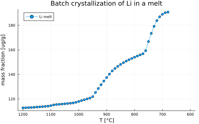

Fractional crystallization

Let's now adapt the previous code to extract cummulates during cooling.

We first need to create an additional Xoxides0 array. This is done in order to be able to update the bulk rock composition. Note that we also create a max_step variable that will record when no melt is stable anymore.

X0          = copy(X)
C0          = copy(C_te)
Xoxides0    = copy(Xoxides)
max_step    = 0

We then compute the fractional crystallization path:

@showprogress for i=1:nsteps
    Out_XY[i]       = single_point_minimization(P, T0[i], data, X=X0, Xoxides=Xoxides0, sys_in=sys_in, name_solvus=true)
    Out_TE_XY[i]    = TE_prediction(Out_XY[i], C0, KDs_dtb, dtb; ZrSat_model = ZrSat_model)
    
    X0              = deepcopy(Out_XY[i].bulk_M_wt)
    Xoxides0        = deepcopy(Out_XY[i].oxides)
    C0              = deepcopy(Out_TE_XY[i].Cliq)

    if Out_XY[i].frac_M_wt == 0.0
        max_step = i
        break;
    end
end

Here X0, Xoxides0 and C0 are updated using melt composition in wt (Out_XY[i].bulk_M_wt), the corresponding oxide list (Out_XY[i].oxides) and the trace element composition of the melt (Out_TE_XY[i].Cliq). Subsequently, the iterations are stopped if the fraction of modeled melt reach 0.0:

if Out_XY[i].frac_M_wt == 0.0
    max_step = i
    break;
end

Plot Li concentration

We can then plot and save the results:

Li_id   = findfirst(isequal("Li"), el)
Li_melt = [Out_TE_XY[i].Cliq[Li_id] for i in 1:max_step if !isnothing(Out_TE_XY[i].Cliq)]
T       = [T0[i] for i in 1:max_step if !isnothing(Out_TE_XY[i].Cliq)]

Note

• Here we extract Li_melt and T up to max_step and not nsteps!

plot(   T,  Li_melt,
        label   = "Li melt",
        xlabel  = "T [°C]",
        ylabel  = "Concentration [ug/g]",
        title   = "Fractional crystallization of Li in a melt",
        marker  =  :circle,
        legend  =  :topleft,
        grid    =  true,
        xflip   =  true)

plot!(size=(640,400))
savefig("MAGEMin_C_LLD_Li.png")

which gives: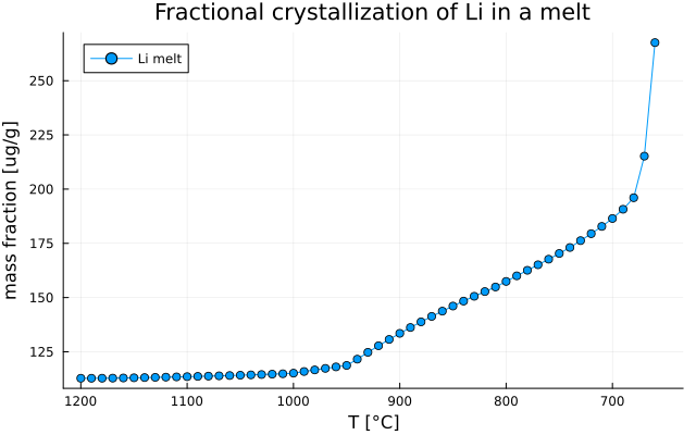

Warning

• When the bulk is first defined the order of the oxides is not necessarily as in the MAGEMin_C output. When updating the bulk in a loop, for instance using the melt composition, we therefore need to retrieve the corresponding oxide ordering.

Plot fraction of zircon

Similarily we can plot the fraction of zircon crystallized from the melt

Zrn_wt = [Out_TE_XY[i].zrc_wt for i in 1:max_step if !isnothing(Out_TE_XY[i].zrc_wt)]
T       = [T0[i] for i in 1:max_step if !isnothing(Out_TE_XY[i].zrc_wt)]

plot(   T,  Zrn_wt,
        label   = "Zrn fraction",
        xlabel  = "T [°C]",
        ylabel  = "wt%",
        title   = "Fractional crystallization of Zrn",
        marker  =  :circle,
        legend  =  :topleft,
        grid    =  true,
        xflip   =  true)

plot!(size=(640,400))
savefig("MAGEMin_C_LLD_Zrn.png")

which gives:

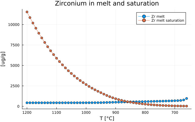
Plot Zr saturation and Zr concentration in melt

We can also plot Zr concentration and saturation of the melt as:

Zr_id   = findfirst(isequal("Zr"), el)
Zr_melt = [Out_TE_XY[i].Cliq[Zr_id] for i in 1:max_step if !isnothing(Out_TE_XY[i].Cliq)]
Zr_melt_sat = [Out_TE_XY[i].Sat_zr_liq for i in 1:max_step if !isnothing(Out_TE_XY[i].Cliq)]
T       = [T0[i] for i in 1:max_step if !isnothing(Out_TE_XY[i].Cliq)]

plot(   T,  Zr_melt,
        label   = "Zr melt",
        xlabel  = "T [°C]",
        ylabel  = "[ug/g]",
        title   = "Zirconium in melt and saturation",
        marker  =  :circle,
        legend  =  :topright,
        grid    =  true,
        xflip   =  true)

plot!(  T,  Zr_melt_sat,
        label   = "Zr melt saturation",
        xlabel  = "T [°C]",
        ylabel  = "[ug/g]",
        title   = "Zirconium in melt and saturation",
        marker  =  :circle,
        legend  =  :topright,
        grid    =  true,
        xflip   =  true)

plot!(size=(640,400))
savefig("MAGEMin_C_LLD_Zr.png")

which gives: