Usage
In order to generate pseudosection (including isochemical phase diagrams) we provide a in-house GUI developped using MATLAB 2020b and tested on MATLAB 2019b.
Specifications
The GUI sends a list of pressure-temperature points to MAGEMin for a specified bulk-rock composition and receives back the stable phase mineral assemblage.
The GUI uses adaptive mesh refinement to refine the reactions lines.
Possibility to save and load pseudosection
Various display options including, stable phases, Gibbs energy, phase fractions, phase compositions (isopleth), densities etc…
KLB-1 Pseudosection tutorial
As a simple tutorial we present the necessary steps needed to produce a pseudosection for KLB-1 peridotite in the KNCFMASTOCr chemical system and from 0.0 to 50 kbar and 800 to 2000°C.
Sarting GUI
Using MATLAB (2019+) launch the GUI within MAGEMin working directory
cd /your_path_to_MAGEMin/MAGEMin_1.x/
run PlotPseudosection.mlapp
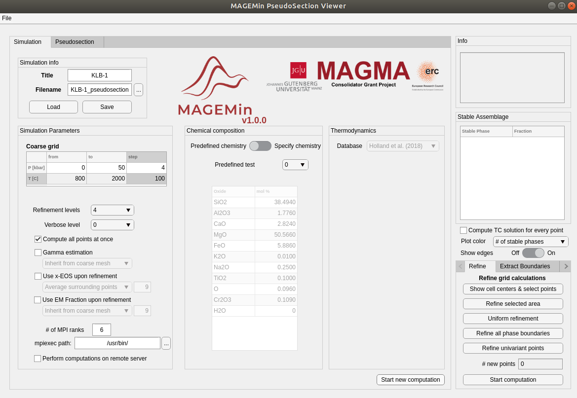
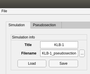
This opens the following window:
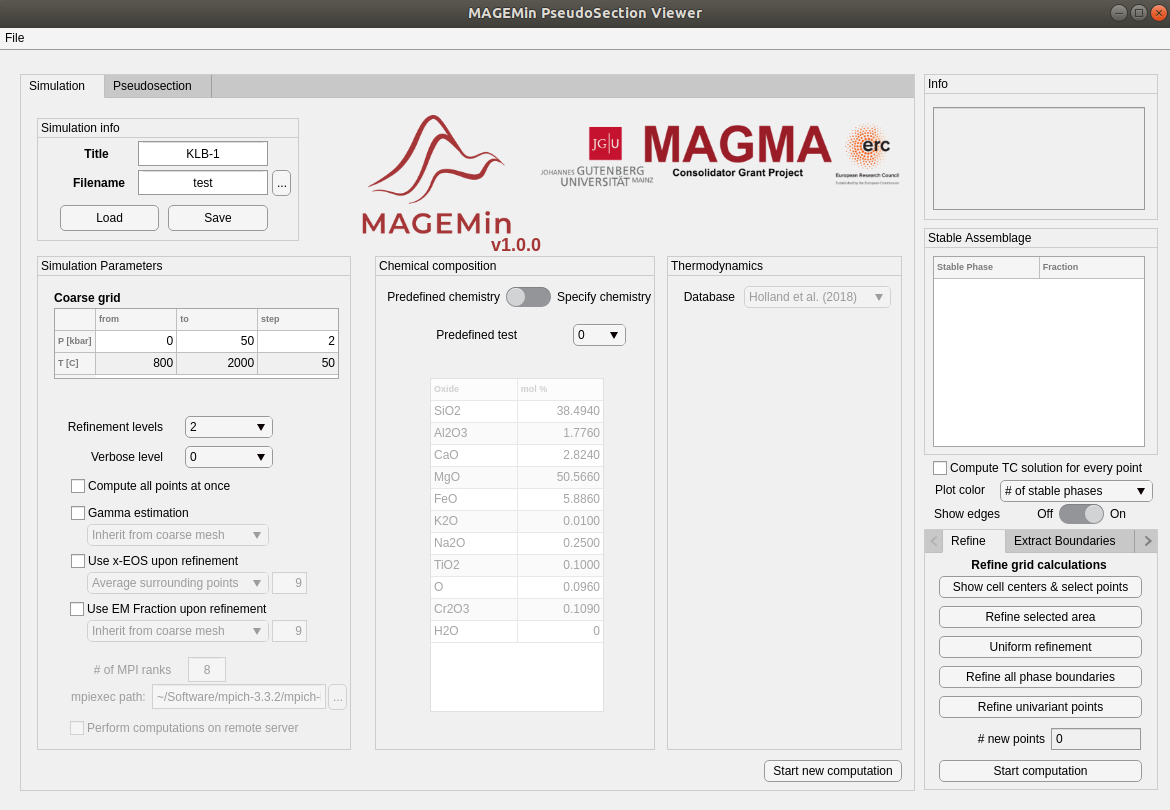
On the displayed window (simulation) you can choose and modifiy several parameters/options. First, you can change the name of the simulation (or save/load a pre-existing simulation)
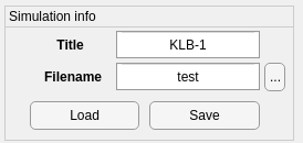
Change the filename from “test” to “KLB-1_pseudosection”
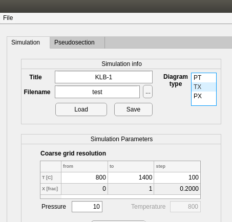
Set P-T conditions
Below you can accept or modify the suggested pressure and temperature range. The step parameter defines the number of points along the pressure and temperature axes.
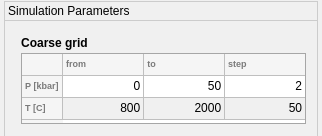
Use the default pressure and temperature range and change the pressure step to 4 kbar and the temperature to 100 °C
Mesh refinement and computation options
Under the P-T range selection, you can access the refinement options and the calculation parameters. By default the refinement is set on 2 levels and the parallel calculation is deactivated.
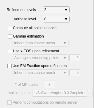
Change the default refinement value to 4
Use default value for verbose
Activate parallel computation by ticking the box “Compute all points at once”
Ticking “Compute all points at once” releases the following options: “# of MPI ranks”, “mpiexec path” and “Perform computations on remote server”
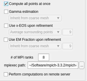
Change “# of MPI ranks” according to the number of core available on your machine
Change “mpiexec path” to your own mpi path e.g. commonly “/usr/bin/” for Linux-based system
Leave “Perform computations on remote server” unticked
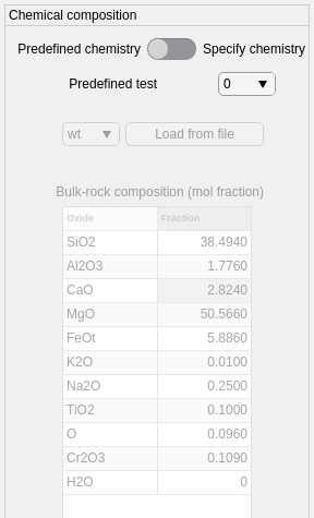
Choose bulk-rock composition
In the middle “Composition” panel you can either specify your own bulk-rock composition or access the in-built list of bulk-rock compositions
To load a custom bulk-rock composition you first need to create a file
your_bulk.dat. The name of the fileyour_bulkwill be used for the name of the pseudosection. The file has to be structured as follow:your_bulk.dat:
SiO2 |
Al2O3 |
CaO |
MgO |
FeO |
Fe2O3 |
K2O |
Na2O |
TiO2 |
Cr2O3 |
H2O |
48.43 |
15.19 |
11.57 |
10.13 |
6.65 |
1.64 |
0.59 |
1.87 |
0.68 |
0.1 |
3.0 |
An example of custom bulk-rock composition is provided in
/examples/bulk1.dat.Note that instead of
Fe2O3, you can directly provideO. If you provideFe2O3the GUI will internally convert it toFeOtandO.
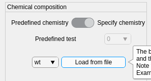
Once the file is created you can load it using the button
Load from file. Note that before loading your bulk-rock composition you first need to select the right system unit[mol or wt]. If the bulk-rock composition you provided is in[wt]it will be automatically converted to[mol], the system unit used in MAGEMin.
For for this tutorial, we will the use default option “pre-defined test 0” (KLB-1 peridotite)
Compute pseudosection
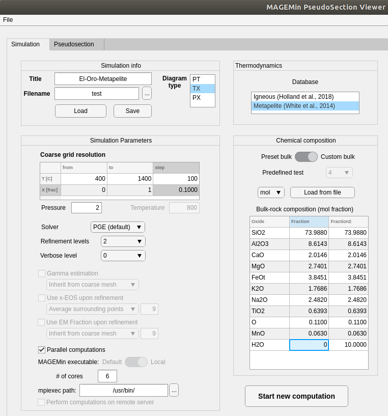
The set of parameters should look like this.
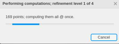
Click on “Start new computation” at the bottom of the “Thermodynamics” panel to launch the computation. If everything is correctly setup it should opens the folloying window
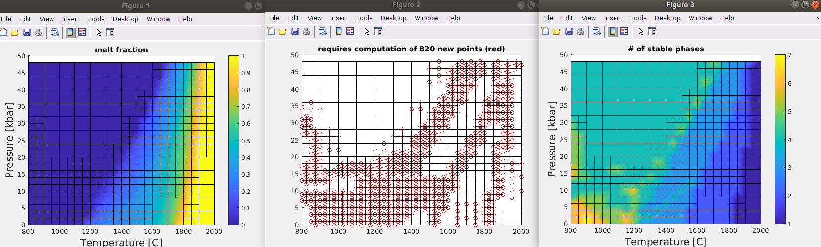
At the end of each refinement step, a set of 3 figures are displayed and updated. They show the “melt fraction”, the “adaptive mesh refinement” and “the number of stable phases”
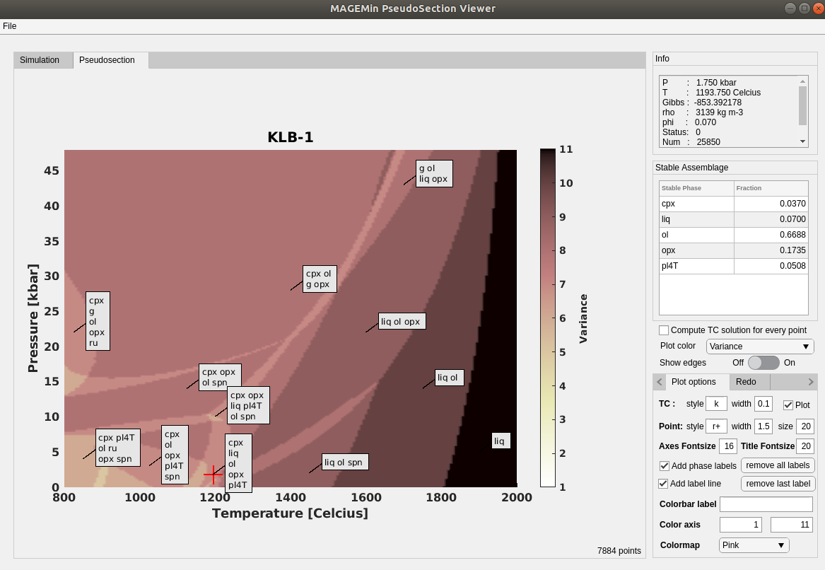
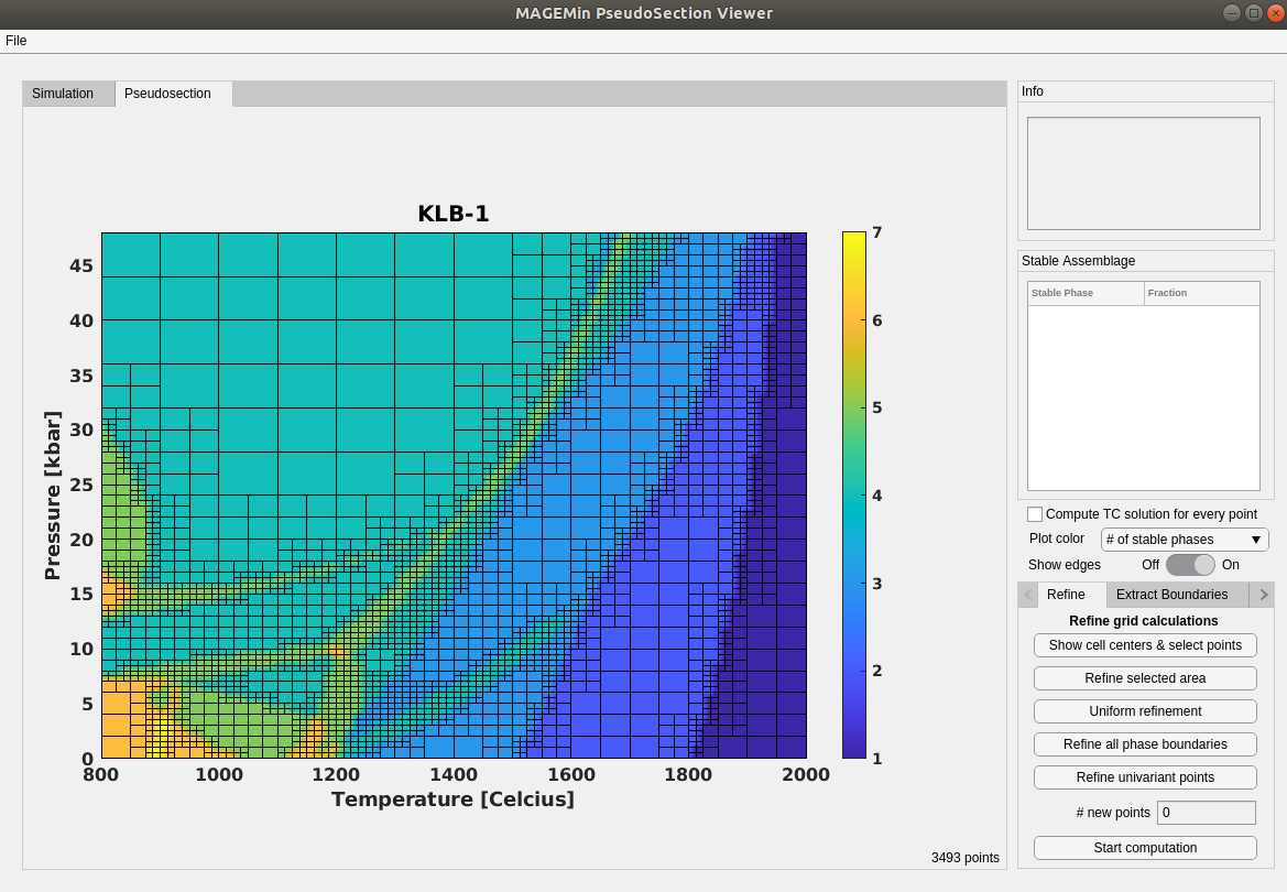
Once the computation is over, the GUI displays the pseudosection. The number of minimization points is shown at the bottom right, for this example “3493 points”. Note that by default the number of stable phases is displayed together wit the mesh refinement grid. Note that, you are in the “Pseudosection” window.
Refine pseudosection
From there you can decide to refine the pseudosection as the resolution is rather low.
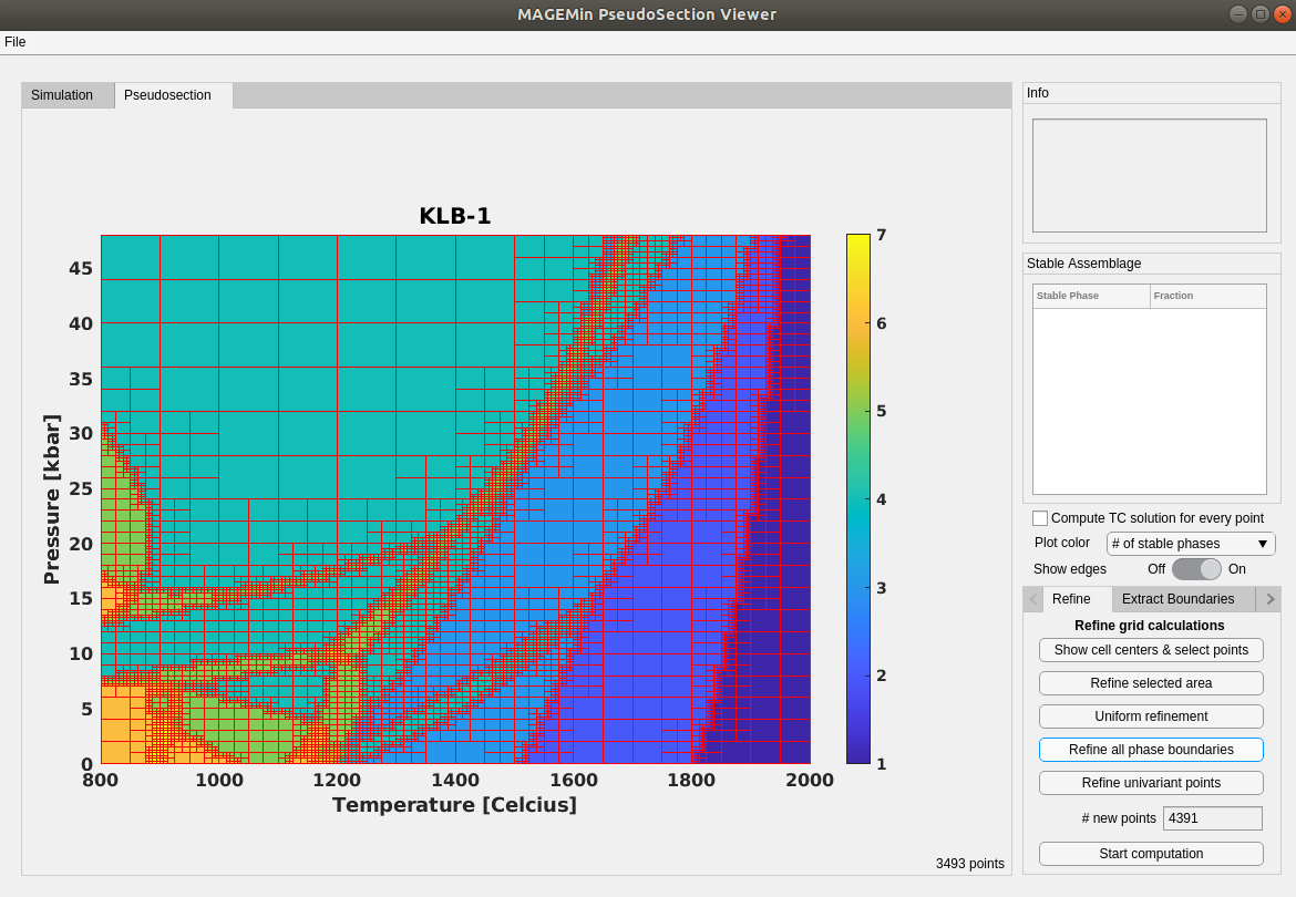
click on “Refine all phase boundaries” in the bottom right corner, and then “Start computation”
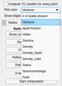
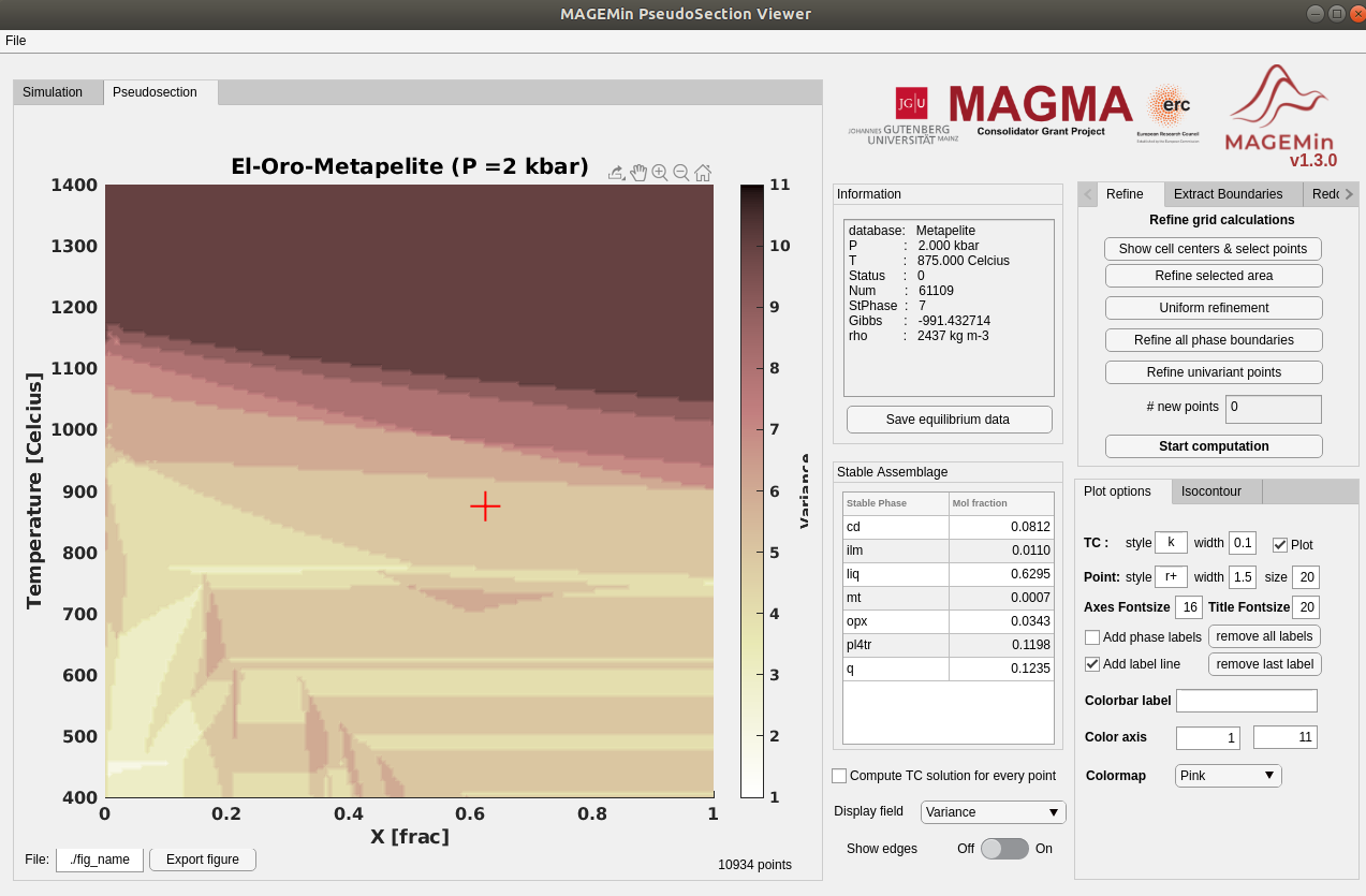
Change displayed field
Upon refinement you can choose to change the field that is displayed
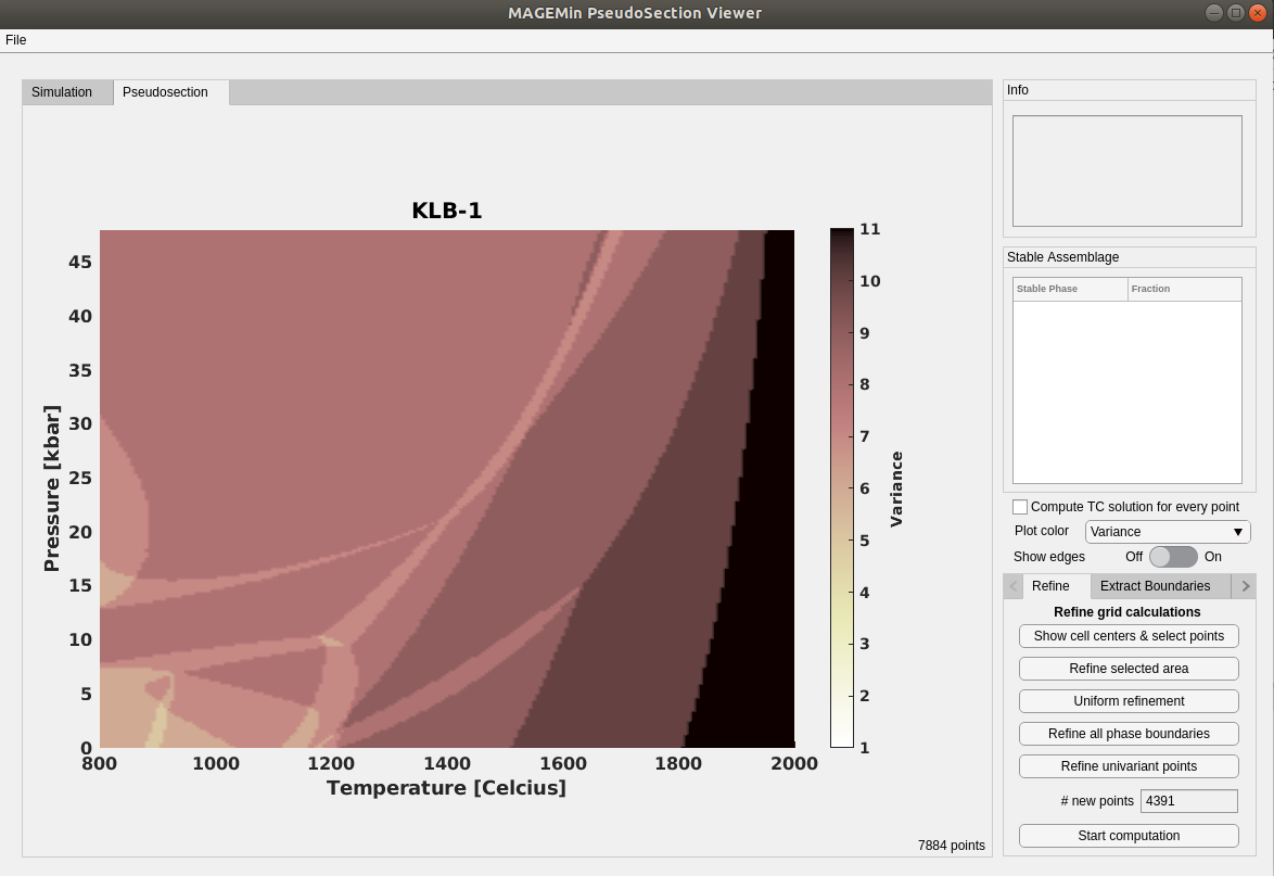
To display the variance click on the “Plot color” menu and select “Variance”
To hide the mesh refinement grid click, set “Show edges” to “Off”, which gives
Display stable phases labels
In the bottom right menu, you can now access the plotting options
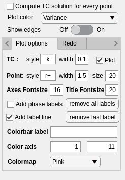
Tick “Add phase labels” and then click on the different fields to display the stable mineral assemblage directly on the grid such as
Note that the label box position, with respect to the field you click on, remains the same e.g. in a top-right position. If you miss-clicked and two boxes overlap, don’t panick, you can always click on “remove last label”, or even “remove all labels” and redo the process
Save pseudosection data
You have the option to save the pseudosection data in a MATLAB “mat” file.
To save the pseudosection data come back to the simulation window, by clicking on the top left “simulation” tab. Then click on “save”. This created the following file
KLB-1_pseudosection.mat
If you close and relaunch the GUI, you can load the saved pseudosection by entering its name in the “Filename” window and click on “load”. Note that loading can potentially take a long time if the pseudosection you saved contains a large number of points
P-X and T-X diagrams
The objective of an P,T-X diagrams is to fix pressure or temperature and vary one or more components of the bulk-rock composition. This section shows how this can be achieved using the GUI of MAGEMin.
Select diagram type
P-X and T-X diagrams can be computed by changing the default option in the top-left corner of the GUI (following snapshot). The fixed pressure can be changed as shown in the bottom-left corner of the following snapshot:
Select compositional range (X)
The compositional range to be explored in a T-X phase diagram can be changed such as:
Here, the
TXdiagram type is first selected, then theMetapelitedatabase is selected. UsingPreset bulkthe predefined test 4 has been activated, thenCustom bulkis instead selected to enable changing the composition of the bulk. Finally the water-content of the first column (Fraction) is changed to 0.0.Setting the desired fixed pressure and temperature range, adjusting the number of refinements to 6, and performing the computation results in:
Note that labeling and iso-contouring works in the same way as for PT diagrams.
Save single point output
If one wants to save the exhaustive informations of one computed grid point this can be achieved (after clicking on a grid point) by clicking on
Save equilibrium datain the information panel. Doing so opens a window allowing you to save the full output as a text file.
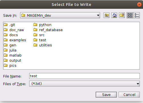
Note that everytime you save the full information about a data point a single calculation is performed and the output format style is the same as for the arg --matlab_out=1
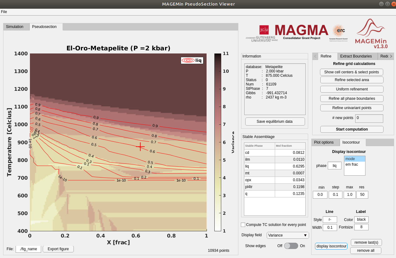
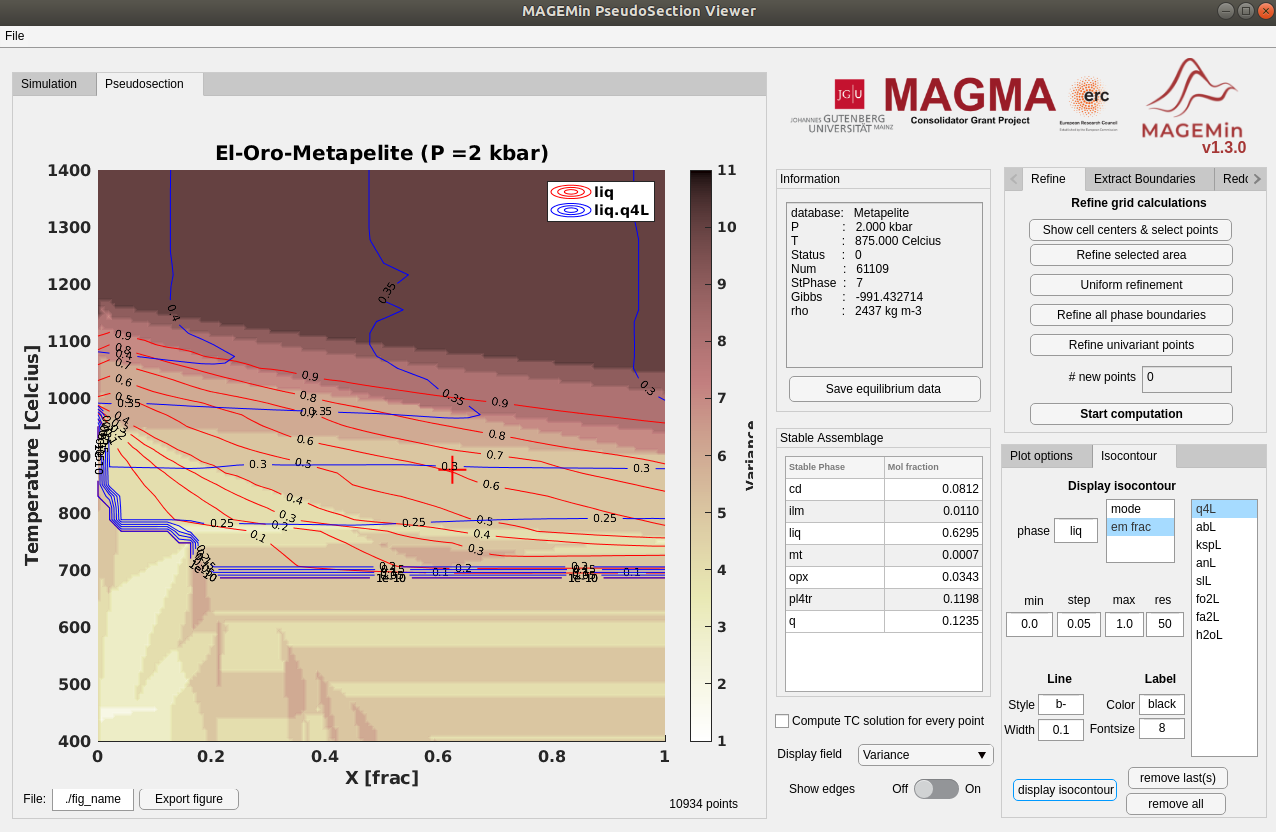
Display iso-contours
Often it is useful to be able to track the lines of constant mineral fraction or end-member proportions. This can be achieved by selecting the
Isocontourpanel in the bottom-right of the GUI.
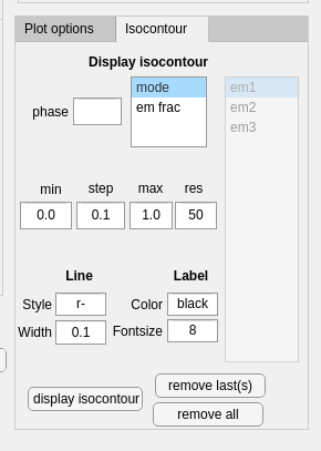
Display phase fraction (mode)
To display isocontours of solution phase fraction first enter the acronym of the desired phase, for instance
liqin thephasecell. Then selectmodeand the desired min, range and max values. Finally hittingdisplay isocontourwill yield:
Multiple isocontour can be added in a similar manner, and deleted using remove last(s) and remove all buttons.
Display end-member fraction
To display isocontours of the end-member fraction of a solution phase, simply select
em fracinstead ofmode. Doing so will open a side panel from which you can select the end-member list. This gives forliq:
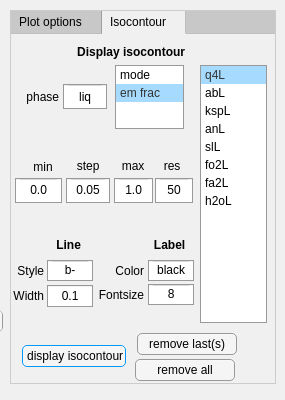
Changing range and color results in:
Save figure (vector)
Computed pahse diagrams including label and isocontour can be saved using the bottom-left
Export figurebutton:
This will save the figure in semi-vectorized format (eps), i.e., that lines labels and contours can be be modified afterward while the colorfield is a bitmap.